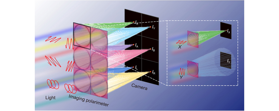
Fig. 1. The schematic of the continuous broadband achromatic imaging polarimeter.The device is composed of 2×3 sub-arrays, each of which can be regarded as an achromatic focusing lens under a specific polarization basis. The focal spots remain at the same plane under different incident lights in 9-12 μm. The schematic in the white frame on the right shows the principle of polarization-dependent phase optimization.

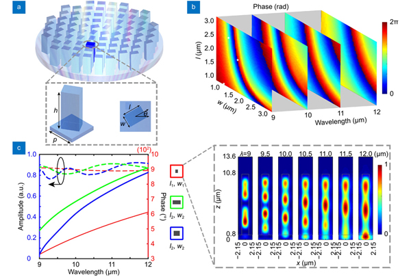
Fig. 2. Optical responses of the unit cells. (a) Schematic illustration of the subwavelength structures. (b) Phase response of the database to X-polarization at discrete sampling wavelengths. (c) The amplitude and phase profiles of the unit cells (l₁, w₁, l₂, w₂, l₃, w₃) are marked with white pentagrams inFig. 2(b). The phase profiles have approximately linear relations with wavelength. The inset is the magnetic energy density profile for the unit cell with l₁ and w₁ at wavelengths 9, 9.5, 10, 10.5, 11, 11.5, and 12 μm. The black line is the outline of the unit cell. The magnetic energy is strongly concentrated in the dielectric nanopillar.

Fig. 3. Simulation results of X- and Y-polarization-sensitive metalenses designed with (a) polarization-dependent optimization method versus (b) conventional design method for X-polarized incident light. The upper diagram shows the intensity distribution in the x-z plane, and the white dashed line is the position of the focal plane. The middle figure is the focal plane intensity profile. The lower part is the normalized intensity profile along the white line.

Fig. 4. Characterization of the polarimeter. (a) Schematic diagram of the process of fabricating polarimeter. (b) Local SEM image of the polarimeter. The inset is an oblique view of the part of the polarimeter, revealing the high aspect ratio of nanopillars. (c) The optical setup for polarimetry. Optical elements: linear polarizer (LP), quarter-wave plate (QWP), metasurface (MS).

Fig. 5. Optical Performances of the broadband achromatic metalenses for linear polarization.(a) TheX andY polarization-sensitive metalenses measured intensity distributions in the x-z plane at sampled incident wavelengths for 9.3, 9.6, 10.3, and 10.6 μm under X polarized incidence. The white dashed lines are the position of the focal plane. (b) The measured focal plane intensity distributions. (c) The extracted focal lengths of the simulation and experiment are a function of wavelength, and all focal lengths are around the target 1 cm. (d) The measured and simulated FWHMs of the focal spots versus the sampled wavelengths. (e) The measured and simulated focusing efficiencies. The blue solids represent the corresponding theoretical results at 9, 9.3, 9.5, 9.6, 10, 10.3, 10.5, 10.6, 11, 11.5, and 12 μm, and the red solids represent the experimental results at 9.3, 9.6, 10.3, and 10.6 μm. Exp.: experiment. Sim.: simulation.

Fig. 6. Characterization results of the polarimeter. Measured intensity distributions at the focal plane and normalized Stokes parameters for different incident polarizations (shown with black arrows) with wavelengths of (a) 9.3 μm, (b) 9.6 μm, (c) 10.3 μm, and (d) 10.6 μm. The theoretically normalized Stokes parameters for X, Y, A, B, L, R, 30º linear polarization and elliptically polarization (the ratio of the major axis to the minor axis is 3 , and the phase difference is 90º) are (1,0, 0), (–1, 0, 0), (0, 1, 0), (0, –1, 0), (0, 0, 1), (0, 0, –1), (0.5, 0.866, 0) and (0.5, 0, 0.866).

Fig. 7. Polarization imaging. (a) Polarization imaging of the polarization mask. (b) Theoretical results (top) and experimental results (bottom) of Stokes parameters S₀–S₃ corresponding to (a). (c) Polarization imaging of the resolution target. (d) Theoretical results (top) and experimental results (bottom) of Stokes parameters S₀–S₃ corresponding to (c).

Table 0. Comparison of the extinction ratio between the polarization-dependent optimization method proposed in this paper and the conventional design method when modulating circular polarization.

Table 0. Comparison of the extinction ratio between the polarization-dependent optimization method proposed in this paper and the conventional design method when modulating linear polarization.