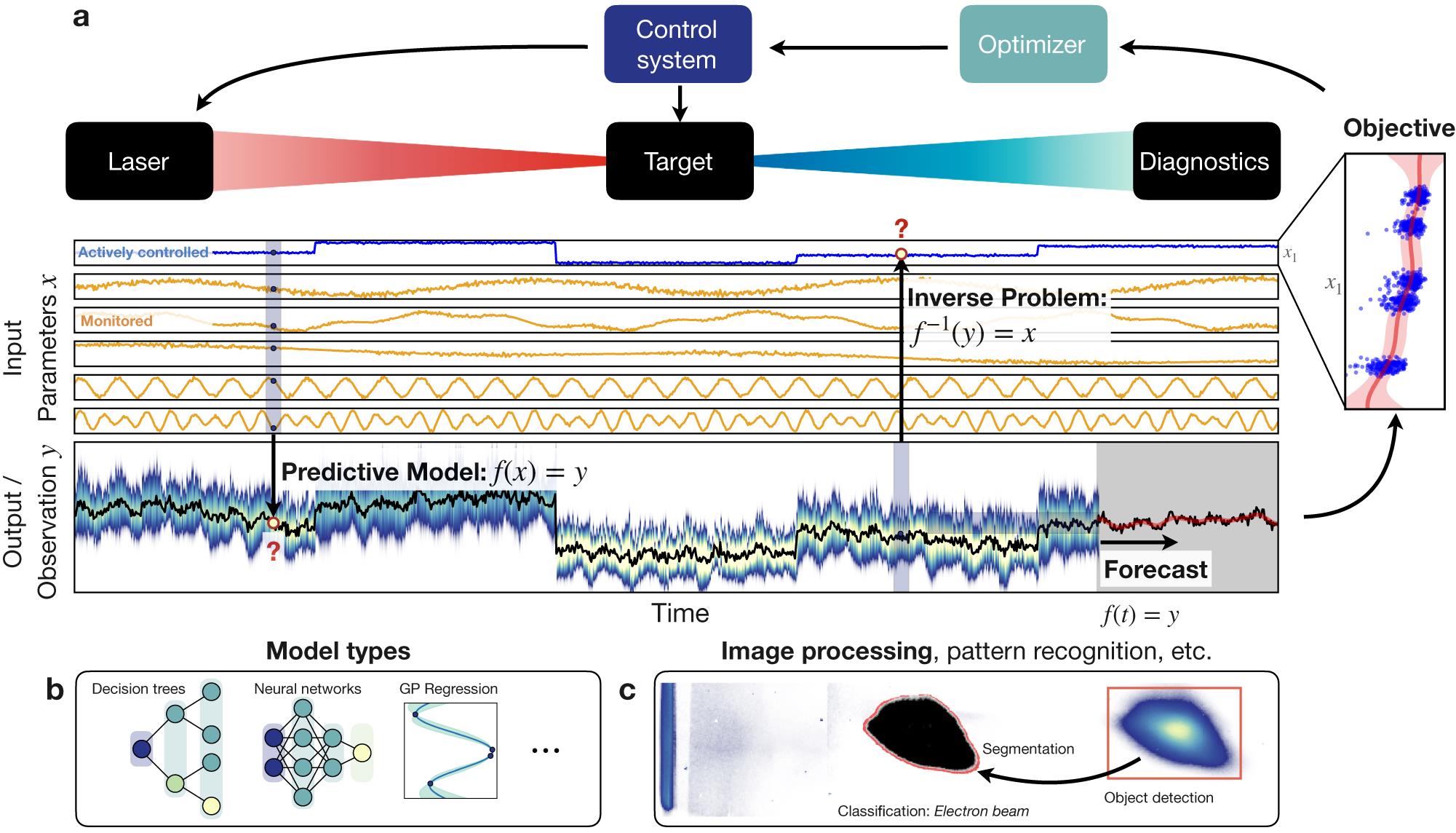
Fig. 1. Overview of some of the machine learning applications discussed in this manuscript. (a) General configuration of laser–plasma interaction setups, applicable to both experiments and simulations. The system will have a number of input parameters of the laser and target. Some of these are known and actively controlled (e.g., laser energy, plasma density), some are monitored and others are unknown and essentially contribute as noise to the observations. Predictive models take the known input parameters and use some models to predict the output . These models are discussed in Section 2.1 and some of them are sketched in (b). Inversely, in some cases one will want to derive the initial conditions from the output. These inverse problems are discussed in Section 3. In other cases one might be interested in a temporal evolution, discussed in Section 2.2. The output from observations or models can be used to optimize certain objectives, which can then be fed back to the control system to adjust the input parameters (see Section 4). Observations may also require further processing, for example, the image processing in (c) to detect patterns or objects. Note that sub-figure (a) is for illustrative purposes only and based on synthetic data.

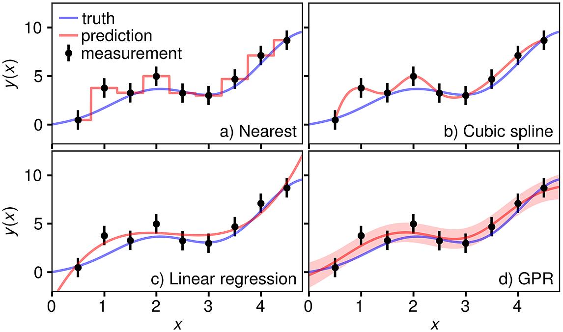
Fig. 2. Illustration of standard approaches to making predictive models in machine learning. The data were sampled from the function with random Gaussian noise, , for which . The data have been fitted by (a) nearest neighbor interpolation, (b) cubic spline interpolation, (c) linear regression of a third-order polynomial and (d) Gaussian process regression.

Fig. 3. Gaussian process regression: illustration of different covariance functions, prior distributions and (fitted) posterior distributions. Left: correlation matrices between two values and using different covariance functions (white noise, radial basis function and periodic). Center: samples of the prior distribution defined by the prior mean and the indicated covariance functions. Note that the sampled functions are depicted with increasing transparency for visual clarity. Right: posterior distribution given observation points sampled from , where is random Gaussian noise with . Note how the variance between observations increases when no noise term is included in the kernel (top row). Within the observation window the fitted kernels show little difference, but outside of it the RBF kernel decays to the mean dependent on the length scale . This can be avoided if there exists prior knowledge about the data that can be encoded in the covariance function, in this case periodicity, as can be seen in the regression using a periodic kernel.

Fig. 4. Sketch of a random forest, an architecture for regression or classification consisting of multiple decision trees, whose individual predictions are combined into an ensemble prediction, for example, via majority voting or averaging.

Fig. 5. Example of gradient boosting with decision trees. Firstly, a decision tree is fitted to the data. In the next step, the residual difference between training data and the prediction of this tree is calculated and used to fit a second decision tree . This process is repeated times, with each new tree learning to correct only the remaining difference to the training data. Data in this example are sampled from the same function as in Figure 2 and each tree has a maximum depth of two decision layers.

Fig. 6. Simplified sketch of some popular neural network architectures. The simplest possible neural network is the perceptron, which consists of an input, which is fed into the neuron that processes the input based on the weights, an individual bias and its activation function. Multiple such layers can be stacked within so-called hidden layers, resulting in the popular multilayer perceptron (or fully connected network). Besides the direct connection between subsequent layers, there are also special connections common in many modern neural network architectures. Examples are the recurrent connection (which feeds the output of the current layer back into the input of the current layer), the convolutional connection (which replaces the direct connection between two layers by the convolutional operation) and the residual connection (which adds the input to the output of the current layer; note that the above illustration is simplified and the layers should be equal in size).

Fig. 7. Real-world example of a multilayer perceptron for beam parameter prediction. (a) The network layout^[29] consists of 15 input neurons, two hidden layers with 30 neurons and three output neurons (charge, mean energy and energy spread). The input is derived from parasitic laser diagnostics (laser pulse energy , central wavelength and spectral bandwidth , longitudinal focus position and Zernike coefficients of the wavefront). Neurons use a nonlinear ReLU activation and 20% of neurons drop out for regularization during training. The (normalized) predictions are compared to the training data to evaluate the accuracy of the model, in this case using the mean absolute error as the loss function. In training, the gradient of the loss function is then propagated back through the network to adjust its weights and biases. (b) Measured and predicted median energy () and (c) measured and predicted energy spread (E), both for a series of 50 consecutive shots. Sub-figures (b) and (c) are adapted from Ref. [29].

Fig. 8. Tomography of a human bone sample using a laser-driven betatron X-ray source. Reconstructed from 180 projections using statistical iterative reconstruction. Based on the data presented by Döpp et al.^[162].

Fig. 9. Deep-learning for inverse problems. Sketch explaining the relation among predictive models, inverse models and fully invertible models.

Fig. 10. Application of the end-to-end reconstruction of a wavefront using a convolutional U-Net architecture^[180]. The spot patterns from a Shack–Hartmann sensor are fed into the network, yielding a high-fidelity prediction. Adapted from Ref. [188].

Fig. 11. Deep unrolling for hyperspectral imaging. The left-hand side displays an example of the coded shot, that is, a spatial-spectral interferogram hypercube randomly sampled onto a 2D sensor. The bottom left shows a magnification of a selected section. On the right-hand side is the corresponding reconstructed spectrally resolved hypercube. Adapted from Ref. [192].

Fig. 12. Pareto front. Illustration of how a multi-objective function acts on a 2D input space and transforms it to an objective space on the right. The entirety of possible input positions is uniquely color-coded on the left and the resulting position in the objective space is shown in the same color on the right. The Pareto-optimal solutions form the Pareto front, indicated on the right, whereas the corresponding set of coordinates in the input space is called the Pareto set. Note that both the Pareto front and Pareto set may be continuously defined locally, but can also contain discontinuities when local maxima become involved. Adapted from Ref. [199].

Fig. 13. Genetic algorithm optimization. (a) Basic working principle of a genetic algorithm. (b) Sketch of a feedback-optimized LWFA via genetic algorithm. (c) Optimized electron beam spatial profiles using different figures of merit. Subfigures (b) and (c) adapted from Ref. [194].

Fig. 14. Bayesian optimization of a laser–plasma X-ray source. (a) The objective function (X-ray counts) as a function of iteration number (top) and the variation of the control parameters (bottom) during optimization. (b) X-ray images obtained for the initial (bottom) and optimal (top) settings. Adapted from Ref. [196].

Fig. 15. Illustration of different optimization strategies for a non-trivial 2D system, here based on a simulated laser wakefield accelerator with laser focus and plasma density as free parameters. The total beam charge, shown as contour lines in plots (a)–(c) serves as the optimization goal. The position of the optimum is marked by a red circle, located at a focus position of and a plasma density of . In panel (a), a grid search strategy with subsequent local optimization using the downhill simplex (Nelder–Mead) algorithm is shown. Panel (b) illustrates differential evolution and (c) is based on Bayesian optimization using the common expected improvement acquisition function. The performance for all three examples is compared in panel (d). It shows the typical behavior that Bayesian optimization needs the least and the grid search requires the most iterations. The local search via the Nelder–Mead algorithm converges within some 20 iterations, but requires a good initial guess (here provided by the grid search). Individual evaluations are shown as shaded dots. Note how the Bayesian optimization starts exploring once it has found the maximum, whereas the evolutionary algorithm tends more towards exploitation around the so-far best value. This behavior is extreme for the local Nelder–Mead optimizer, which only aims to exploit and maximize to local optimum.

Fig. 16. Sketch of deep reinforcement learning. The agent, which consists of a policy and a learning algorithm that updates the policy, sends an action to the environment. In the case of model-based reinforcement learning, the action is sent to the model, which is then applied to the environment. Upon the action to the environment, an observation is made and sent back to the agent as a reward. The reward is used to update the policy via the learning algorithm in the agent, which leads to an action in the next iteration.

Fig. 17. Data treatment using a Gaussian mixture model (GMM). Top: 10 consecutive shots from a laser wakefield accelerator. Middle: the same shots using a GMM to isolate the spectral peak at around 250 MeV. Bottom: average spectra with and without GMM cleaning. Adapted from Ref. [245].

Fig. 18. Correlogram – a visualization of the correlation matrix – of different variables versus yield at the NIF. Color indicates the value of the correlation coefficient. In this particular representation the correlation is also encoded in the shape and angle of the ellipses, helping intuitive understanding. The strongest correlation to the fusion yield is observed with the implosion velocity and the ion temperature . There is also a clear anti-correlation observable between the down-scattered ratio (DSR) and and, in accordance with the previously stated correlation of and yield, a weak anti-correlation of the DSR and yield. Note that all variables perfectly correlate with themselves by definition. Plot was generated based on data presented by Hsu et al.^[96]. Further explanation (labels, etc.) can be found therein.

Fig. 19. Illustration of common computer vision tasks. (a) Classification is used to assign (multiple) labels to data. (b) Detection goes a step further and adds bounding boxes. (c) Segmentation provides pixel maps with exact boundaries of the object or feature.

Fig. 20. Application of object detection to a few-cycle shadowgram of a plasma wave: the plasma wave, the shadowgram of a hydrodynamic shock and the diffraction pattern caused by dust are correctly identified by the object detector and located with bounding boxes. Adapted from Ref. [273].

Table 1. Summary of a few representative papers on machine-learning-aided optimization in the context of laser–plasma acceleration and high-power laser experiments.

Table 2. Summary of papers used as application examples in this review, sorted by year for each section.