
Andreas Döpp, Christoph Eberle, Sunny Howard, Faran Irshad, Jinpu Lin, Matthew Streeter, "Data-driven science and machine learning methods in laser–plasma physics," High Power Laser Sci. Eng. 11, 05000e55 (2023)
- High Power Laser Science and Engineering
- Vol. 11, Issue 5, 05000e55 (2023)
Abstract
1 Introduction
1.1 Laser–plasma physics
Over the past decades, the development of increasingly powerful laser systems[1,2] has enabled the study of light–matter interaction across many regimes. Of particular interest is the interaction of intense laser pulses with plasma, which is characterized by strong nonlinearities that occur across many scales in space and time[3,4]. These laser–plasma interactions are of interest both for fundamental physics research and as emerging technologies for potentially disruptive applications.
Regarding fundamental research, high-power lasers have, for instance, been used to study transitions from classical electrodynamics to quantum electrodynamics (QED) via the radiation reaction, where a particle’s backreaction to its radiation field manifests itself in an additional force[5–7]. Recent proposals to extend intensities to the Schwinger limit[8], where the electric field strength of the light is comparable to the Coulomb field, could allow the study of novel phenomena expected to occur due to a breakdown of perturbation theory. In an only slightly less extreme case, high-energy density physics (HEDP)[9] research uses lasers for the production and study of states of matter that cannot be reached otherwise in terrestrial laboratories. This includes creating and investigating material under extreme pressures and temperatures, leading to exotic states such as warm–dense matter[10–12].
Apart from the fundamental interest, there is also considerable interest in developing novel applications that are enabled by these laser–plasma interactions. Two particularly promising application areas have emerged over the past decades, namely the production of high-energy radiation beams (electrons, positrons, ions, X-rays, gamma-rays) and laser-driven fusion.
Sign up for High Power Laser Science and Engineering TOC. Get the latest issue of High Power Laser Science and Engineering delivered right to you!Sign up now
Laser–plasma acceleration (LPA) aims to accelerate charged particles to high energies over short distances by inducing charge separation in the plasma, for example, in the form of plasma waves to accelerate electrons or by stripping electrons from thin-foil targets to accelerate ions. The former scenario is called laser wakefield acceleration (LWFA)[13–15]. Here a high-power laser propagates through a tenuous plasma and drives a plasma wave, which can take the shape of a spherical ion cavity directly behind the laser. The fields within this so-called bubble typically reach around 100 GV/m, allowing LWFA to accelerate electrons from rest to GeV energies within centimeters[16–21]. While initial experiments were single-shot in nature and with significant shot-to-shot variations, the performance of LWFA has drastically increased in recent years. Particularly worth mentioning in this regard are the pioneering works on LWFA at the kHz-level repetition rate, starting with an early demonstration in 2013[22] and in the following years mostly developed by Faure et al.[23], Rovige et al.[24] and Salehi et al.[25], as well as the day-long stable operation achieved by Maier et al.[26]. As a result of these efforts, typical experimental datasets in publications have significantly increased in size. To give an example, first studies on the so-called beamloading effect in LWFA were done on sets of tens of shots[27], whereas newer studies include hundreds of shots[28] or, most recently, thousands of shots[29].
Laser-driven accelerators can also function as bright radiation sources via the processes of bremsstrahlung emission[30,31], betatron radiation[32,33] and Compton scattering[34–36]. These sources have been used for a variety of proof-of-concept applications[37], ranging from spectroscopy studies of warm–dense matter[10] and over imaging[38,39] to X-ray computed tomography (CT)[40–43]. It has also recently been demonstrated that LWFA can produce electron beams with sufficiently high beam quality to drive free-electron lasers (FELs)[44,45], offering a potential alternative driver for next generation light sources[46].
Laser-ion acceleration[47,48] uses similar laser systems as LWFA, but typically operates with more tightly focused beams to reach even higher intensities. Here the goal is to separate a population of electrons from the ions and then use this electron cloud to strip ions from the target. The ions are accelerated to high energies by the fields that are generated by the charge separation process. This method has been used to accelerate ions to energies of a few tens of MeV/u in recent years. In an alternative scheme, radiation pressure acceleration[49,50], the laser field is used to directly accelerate a target. Even though it uses the same or similar lasers, ion acceleration typically operates at much lower repetition rate because of its thin targets, which are not as easily replenished as gas-based plasma sources used in LWFA. Recent target design focuses on the mitigation of this issue, for instance using cryogenic jets[51–54] or liquid crystals[55].
Another application of potentially high societal relevance is laser-driven inertial confinement fusion (ICF)[56,57], where the aim is to induce fusion by heating matter to extremely high temperatures through laser–plasma interaction. As the name suggests, confinement is reached via the inertia of the plasma, which is orders of magnitude larger than the thermal energy. To achieve spatially homogenous heating that can penetrate deep into the fusion target, researchers commonly resort to driving the ignition process indirectly. In this method, light is focused into an empty cylindrical cavity, called a hohlraum, which is used to radiate a nearly isotropic blackbody spectrum that extends into the X-ray regime and is subsequently absorbed by the imploding capsule[58]. In contrast to this, direct-drive methods aim to directly drive the thermonuclear fusion process[59]. In this case, the laser is focused directly onto the fuel capsule. Direct-drive poses some challenges that are not present in indirect-drive schemes. For instance, the light has to penetrate through the high-density plasma shell surrounding the capsule and the illumination is less homogeneous, because of which the compressed target can be subject to large hydrodynamic instabilities. Advanced ignition schemes aim to separate compression of the thermonuclear fuel from triggering the ignition process. Examples are fast ignition[60], which uses the high-intensity laser pulse to directly heat the compressed and dense fusion target, and shock ignition[61], which uses a shock wave to compress the target. Recently, the first ICF experiment at the National Ignition Facility (NIF) has reported reaching the burning-plasma state via the combination of indirect-drive with advanced target design[62]. This breakthrough has re-enforced scientific and commercial interest in ICF, which is now also being pursued by a number of start-up companies.
1.2 Why data-driven techniques?
In recent years, data-driven methods and machine learning have been applied to a wide range of physics problems[63], including for instance quantum physics[64,65], particle physics[66], condensed matter physics[67], electron microscopy[68] and fluid dynamics[69]. In comparison, its use in laser–plasma physics is still in its infancy and is curiously driven by both data abundance and data scarcity. Regarding the former, fast developments in both laser technology[70] and plasma targetry[71–74] nowadays permit the operation of laser–plasma experiments – in particular laser–plasma accelerators – at joule-level energies and multi-Hz to kHz repetition rates[75–79]. The vast amounts of data generated by these experiments can be used to develop data-driven models, which are then employed in lieu of conventional theoretical or empirical approaches, or to augment them. In contrast, laser systems used for inertial fusion research produce MJ-level laser pulses and operate at repetition rates as low as one shot per day. With such a sparse number of independent experimental runs, data-driven models are used to extract as much information as possible from the existing data or combine them with other information sources, such as simulations.
The success of all of the above applications depends on the precise control of a complex nonlinear system. In order to optimize and control the process of laser–plasma interaction, it is essential to understand the underlying physics and to be able to model the complex plasma response to an applied laser pulse. However, this is complicated by the fact that it is a strongly nonlinear, multi-scale, multi-physics phenomenon. While analytical and numerical models have been essential tools for understanding laser–plasma interactions, they have several limitations. Firstly, analytical models are often limited to low-order approximations and therefore cannot accurately predict the behavior of complex laser–plasma systems. Secondly, accurate numerical simulations require immense computational resources, often millions of core hours, which limits their use for optimizing and controlling real-world laser–plasma experiments. In addition, the huge range of temporal and spatial scales means that in practice many physical processes (ionization, particle collisions, etc.) can only be treated approximately in large-scale numerical simulations. Because of this, one active area of research is to automatically extract knowledge from data in order to build faster computational models that can be used for prediction, optimization, classification and other tasks.
Another important problem is that the diagnostics employed in laser–plasma physics experiments typically only provide incomplete and insufficient information about the interaction, and key properties must be inferred from the limited set of available observables. Such inverse problems can be hard to solve, especially when some information is lost in the measurement process and the problem becomes ill-posed. Modern methods, such as compressed sensing (CS) and deep learning, are strong candidates to facilitate the solution of such problems and thus retrieve so-far elusive information from experiments.
The goal of this review is to summarize the rapid, recent developments of data-driven science and machine learning in laser–plasma physics, with particular emphasis on LPA, and to provide guidance for novices regarding the tools available for specific applications. We would like to start with a disclaimer that the lines between machine learning and other methods are often blurred.1 Given the multitude of often competing subdivisions, we have chosen to organize this review based on a few broad classes of problems that we believe to have highest relevance for laser–plasma physics and its applications. These problems are modeling and prediction (Section 2), inverse problems (Section 3), optimization (Section 4), unsupervised learning for data analysis (Section 5) and, lastly, image analysis with supervised learning techniques (Section 6). Partial overlap between these applications and the tools used is unavoidable and is where possible indicated via cross-references. This is particularly true in the case of neural networks, which have found a broad usage across applications. Each section includes introductions to the most common techniques that address the problems outlined above. We explicitly include what can be considered as ‘classical’ data-driven techniques in order to provide a better context for more recent methods. Furthermore, examples for implementations of specific techniques in laser–plasma physics and related fields are highlighted in separate text boxes. We hope that these will help the reader to get a better idea of which methods might be most adequate for their own research. An overview of the basic application areas is shown in Figure 1.
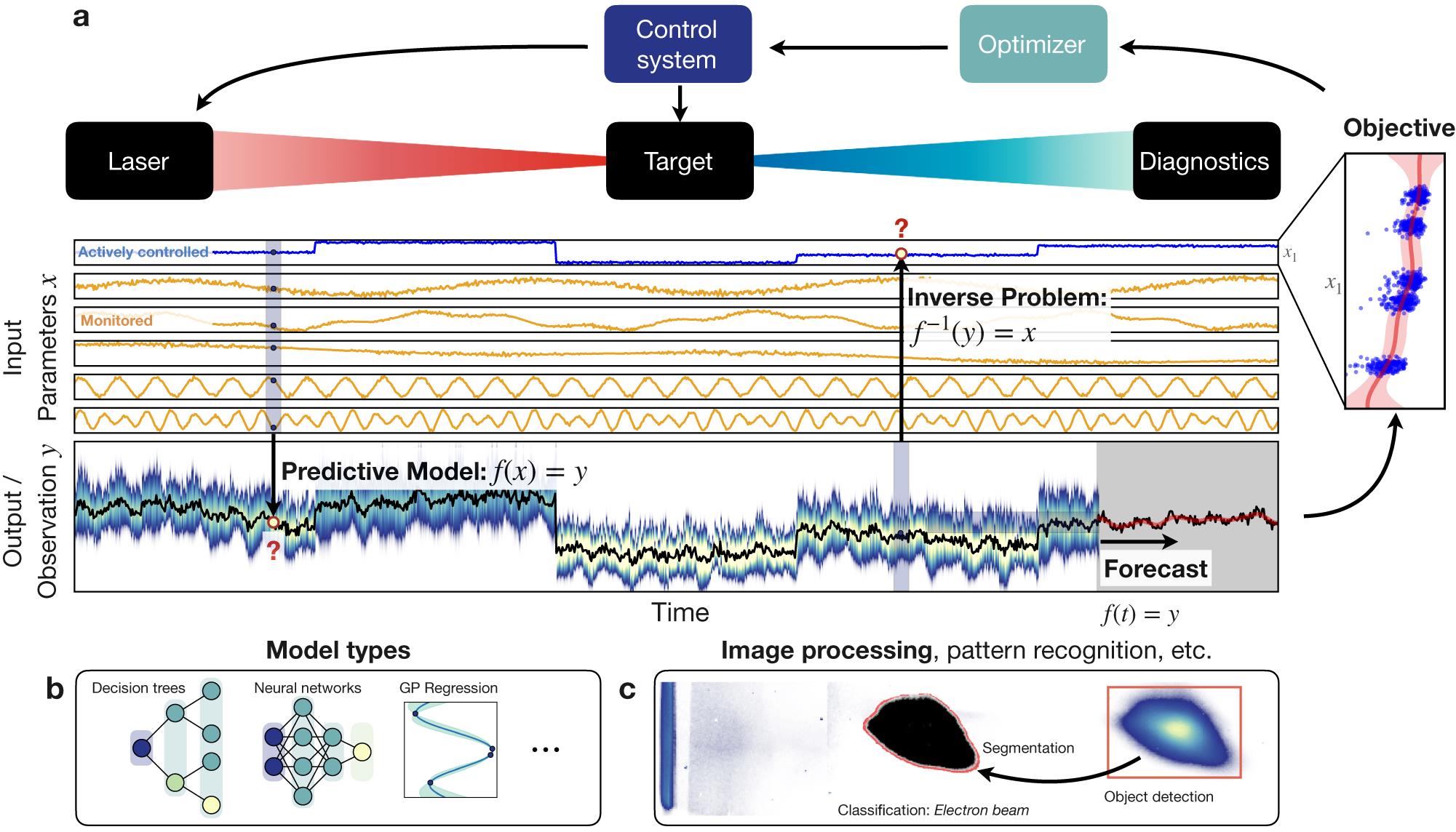
Figure 1.Overview of some of the machine learning applications discussed in this manuscript. (a) General configuration of laser–plasma interaction setups, applicable to both experiments and simulations. The system will have a number of input parameters of the laser and target. Some of these are known and actively controlled (e.g., laser energy, plasma density), some are monitored and others are unknown and essentially contribute as noise to the observations. Predictive models take the known input parameters  and use some models to predict the output
  . These models are discussed in
To maintain brevity and readability, some generalizations and simplifications are made. For detailed descriptions and strict definitions of methods, the reader may kindly refer to the references given throughout the text. Furthermore, we would like to draw the reader’s attention to some recent reviews on the application of machine learning techniques in the related fields of plasma physics[80–82], ultra-fast optics[83] and HEDP[84].
2 Modeling and prediction
Many real-life and simulated systems are expensive to evaluate in terms of time, money or other limited resources. This is particularly true for laser–plasma physics, which either hinges on the limited access to high-power laser facilities or requires high-performance computing to accurately model the ultra-fast laser–plasma interaction. It is therefore desirable to find models of the system, sometimes called digital twins[85], which are comparatively cheap to evaluate and whose predictions can be used for extensive analyses. In engineering and especially in the context of model-based optimization (see Section 4), such lightweight models are often referred to as surrogate models. Reduced-order models feature fewer degrees of freedom than the original system, which is often achieved using methods of dimensionality reduction (see Section 5.3).
The general challenge in modeling is to find a good approximation of
The predictive models discussed in Section 2.1 below are mostly used to interpolate between training data, whereas the related problem of forecasting (Section 2.2) explicitly deals with the issue of extrapolating from existing data to new, so-far unseen data. In Section 2.3 we briefly discuss how models can be used to provide direct feedback for laser–plasma experiments.
2.1 Predictive models
In this section, we describe some of the most common ways to create predictive models, starting with the ‘classic’ approaches of spline interpolation and polynomial regression, before discussing some modern machine learning techniques.
2.1.1 Spline interpolation
The simplest way of constructing a model for a system, be it a real-world system or some complex simulation, is to use a set of
![]()
Figure 2.Illustration of standard approaches to making predictive models in machine learning. The data were sampled from the function  with random Gaussian noise,
  , for which
  . The data have been fitted by (a) nearest neighbor interpolation, (b) cubic spline interpolation, (c) linear regression of a third-order polynomial and (d) Gaussian process regression.
2.1.2 Regression
In some specific cases the shortcomings of interpolation approaches can be addressed by using regression models. For instance, simple systems can often be described using a polynomial model, where the coefficients of the polynomial are determined via a least-squares fit (see Figure 2(c)), that is, minimizing the sum of the squares of the difference between the predicted and observed data. The results are generally improved by including more terms in the polynomial but this can lead to overfitting – a situation where the model describes the noise in the data better than the actual trends, and consequently will not generalize well to unseen data. Regression is not restricted to polynomials, but may use all kinds of mathematical models, often motivated by a known underlying physics model. Crucially, any regression model requires the prior definition of a function to be fitted, thus posing constraints on the relationships that can be modeled. In practice this is one of the main problems with this approach, as complex systems can scarcely be described using simple analytical models. Before using these models, it is thus important to verify their validity, for example, using a measure for the goodness of fit such as the correlation coefficient
2.1.3 Probabilistic models
The field of probabilistic modeling relies on the assumption that the relation between the observed data and the underlying system is stochastic in nature. This means that the observed data are assumed to be drawn from a probability distribution for each set of input parameters to a generative model. Inversely, one can use statistical methods to infer the parameters that best explain the observed data. We will discuss such inference problems in more detail in the context of solving (ill-posed) inverse problems in Section 3.2.
Probabilistic models can generally be divided into two methodologies, frequentist and Bayesian. At the heart of the frequentist approach lies the concept of likelihood,
The optimum can be found using a variety of optimization methods, for example, gradient descent, which are described in more detail in Section 4. A simple example is the use of MLE for parameter estimation in regression problems. In the case in which the error
The MLE is often seen as the simplest and most practical approach to probabilistic modeling. One advantage is that it does not require any a priori assumptions about the model parameters, rather only about the probability distributions of the data. However, this can also be a drawback if useful prior knowledge of the model parameters is available. In this case one would turn to Bayesian statistics. Here one assesses information about the probability that a hypothesis about the parameter values
As mentioned above, a particular strength of the Bayesian approach is that we can encode a priori information in the prior distribution. Taking the example of polynomial regression, we could, for instance, set a priori distribution
2.1.4 Gaussian process regression
A popular version of Bayesian probabilistic modeling is GP regression[87,88]. This kind of modeling was pioneered in geostatistics in the context of mining exploration and is historically also referred to as kriging, after the South African engineer Danie G. Krige, who invented the method in the 1950s. Conceptually, one can think of it as loosely related to the spline interpolation method, as it is also locally ‘interpolates’ the training points. Compared to splines and conventional regression methods, kriging has a number of advantages. Being a regression method, kriging can deal with noisy training points, as seen in experimental data. At the same time, the use of GPs involves minimal assumptions and can in principle model any kind of function. Lastly, the ‘interpolation’ is done in a probabilistic way, that is, a probability distribution is assigned to the function values at unknown positions (see Figure 2(d)). This allows for quantifying the uncertainty of the prediction. These features make kriging an attractive method for the construction of surrogate models for complex systems for which only a limited number of the function evaluations is possible, for example, due to the long runtime of the system or the high costs of the function evaluations. GP regression forms the backbone of most implementations of Bayesian optimization (BO), which we will discuss in Section 4.5, including examples for potential use cases.
Mathematically speaking, a GP is an infinite collection of normal random variables, where each finite subset is jointly normally distributed. The mean vector and covariance matrix of the multivariate normal distribution are thereby generalized to the mean function
A GP can be written in the following form:
The mean function
It is possible to encode prior knowledge by choosing a specialized kernel that imposes certain restrictions on the model. A variety of such kernels exist. For instance, the periodic kernel (also known as exp-sine-square kernel) given by the following:
A useful property of kernels is the generation of new kernels through the addition or multiplication of existing kernels[89]. This property provides another way to leverage prior information about the form of the function to increase the predictive accuracy of the model. For instance, measurement errors incorporated into the model by adding a Gaussian white noise kernel, as for instance done in Figure 2.
Figure 3 visualizes the covariance functions and their influence on the result of GP regression. This includes correlation matrices for the three covariance functions discussed above (white noise, RBF and periodic kernels). Once the mean and the covariance functions are fully defined, we can use training points for regression, that is, fit the GP and kernel parameters to the data and obtain the posterior distribution (see the right-hand panel of Figure 3).
![]()
Figure 3.Gaussian process regression: illustration of different covariance functions, prior distributions and (fitted) posterior distributions.  and
and  using different covariance functions (white noise, radial basis function and periodic).
  and the indicated covariance functions. Note that the sampled functions are depicted with increasing transparency for visual clarity.
  , where
  is random Gaussian noise with
  . Note how the variance between observations increases when no noise term is included in the kernel (top row). Within the observation window the fitted kernels show little difference, but outside of it the RBF kernel decays to the mean
  dependent on the length scale
  . This can be avoided if there exists prior knowledge about the data that can be encoded in the covariance function, in this case periodicity, as can be seen in the regression using a periodic kernel.
![]()
Figure 4.Sketch of a random forest, an architecture for regression or classification consisting of multiple decision trees, whose individual predictions are combined into an ensemble prediction, for example, via majority voting or averaging.
2.1.5 Decision trees and forests
A decision tree is a general-purpose machine learning method that learns a tree-like model of decision rules from the data to make predictions[90]. It works by splitting the dataset recursively into smaller groups, called nodes. Each node represents a decision point, and the tree branches out from the node according to the decisions that are made. The leaves of the tree represent the final prediction; see Figure 4 for an illustration. This can be either a categorical value in classification tasks (see Section 6) or a numerical value prediction in regression tasks. An advantage of this approach is that it can learn nonlinear relationships in data without having to specify them.
To generate a decision tree one starts at the root of the tree and determines a decision node such that it optimizes an underlying decision metric, such as the MSE in regression settings or entropy and information gain in a classification setting. At each decision point the dataset is split and subsequently the metric is re-evaluated for the resulting groups, generating the next layer of decision nodes. This process is repeated until the leaves are reached. The more decision layers are used, called the depth of the tree, the more complex relationships can be modeled.
Decision trees are easy to implement and can provide accurate predictions even for large datasets. However, with an increasing number of decision layers they may become computationally expensive and may overfit the data, the latter being in particular a problem with noisy data. One method to address overfitting is called pruning, where branches from the tree that do not improve the performance are removed. Another effective method is to use decision-tree-based ensemble algorithms instead of a single decision tree.
![]()
Figure 5.Example of gradient boosting with decision trees. Firstly, a decision tree  is fitted to the data. In the next step, the residual difference between training data and the prediction of this tree is calculated and used to fit a second decision tree
  . This process is repeated
  times, with each new tree
  learning to correct only the remaining difference to the training data. Data in this example are sampled from the same function as in
One example of such an algorithm is the random forest, an ensemble algorithm that uses bootstrap aggregating or bagging to fit trees to random subsets of the data and the predictions of individually fitted decision trees are combined by majority vote or average to obtain a more accurate prediction. Another type of ensemble algorithms is boosting, where the trees are trained sequentially and each tries to correct its predecessor. A popular implementation is AdaBoost[91], where the weights of the samples are changed according to the success of the predictions of the previous trees. Gradient boosting methods[92,93] also use the concept of sequentially adding predictors, but while AdaBoost adjusts weights according to the residuals of each prediction, gradient boosting methods fit new residual trees to the remaining differences at each step (see Figure 5 for an example).
Compared to other machine learning algorithms, a great advantage of a decision tree is its explicitness in data analysis, especially in nonlinear high-dimensional problems. By splitting the dataset into branches, the decision tree naturally reveals the importance of each variable regarding the decision metric. This is in contrast to ‘black-box’ models, such as those created by neural networks, which must be interpreted by post hoc analysis.
Decision trees can also be used to seed neural networks by giving the initial weight parameters to train a deep neural network. Examples of using a decision tree as an initializer are the deep jointly-informed neural networks (DJINNs) developed by Humbird et al.[
2.1.6 Neural networks
Neural networks offer a versatile framework for fitting of arbitrary functions by training of a network of connected nodes or neurons, which are loosely inspired by biological neurons. In the case of a fully connected neural network, historically called a multilayer perceptron, the inputs to one node are the outputs of all of the nodes from the preceding layer. The very first layer is simply all of the inputs for the function to be modeled, and the very last layer is the function outputs. One of the very attractive properties of neural networks is the capacity to have many outputs and inputs, each of which can be multi-dimensional. The weighting of each connection
One of the simplest, but also most common, activation functions is the rectified linear unit (ReLU), which is defined as follows:
The function argument
The training is performed iteratively by passing corresponding input–output pairs to the network and comparing the true outputs to those given by the network to calculate the loss function. This is often chosen to be the MSE between the model output and the reference from the training data, but many other types of loss functions are also used (see Section 4.1.1) and the choice of loss function strongly affects the model’s training. The loss is then used to modify the weights and biases via an algorithm known as ‘back-propagation’[99]. Here the gradient of the loss function is calculated with respect to the weights and biases via the chain rule. One can then optimize the parameters using, for instance, stochastic gradient descent (SGD) or Adam (adaptive moment estimation)[100].
A number of hyperparameters are used to control the training process. Typical ones include the following: the number of epochs – the number of times the model sees each data point; the batch size – the number of data points the model sees before updating its gradients; and the learning rate – a factor determining the magnitude of the update to the gradient. Each factor can have a critical effect on the training of the model.
![]()
Figure 6.Simplified sketch of some popular neural network architectures. The simplest possible neural network is the perceptron, which consists of an input, which is fed into the neuron that processes the input based on the weights, an individual bias and its activation function. Multiple such layers can be stacked within so-called hidden layers, resulting in the popular multilayer perceptron (or fully connected network). Besides the direct connection between subsequent layers, there are also special connections common in many modern neural network architectures. Examples are the recurrent connection (which feeds the output of the current layer back into the input of the current layer), the convolutional connection (which replaces the direct connection between two layers by the convolutional operation) and the residual connection (which adds the input to the output of the current layer; note that the above illustration is simplified and the layers should be equal in size).
In the training process, the weights and biases are optimized in order to best approximate the function for converting the inputs into the corresponding outputs. The resulting model will yield an approximation for the unknown function
Common methods to combat overfitting include early stopping, that is, terminating the training process once the validation loss stagnates; or the use of dropout layers to randomly switch off some fraction of the network connections for each batch of the training process, thereby preventing the network from learning random noise by reducing its capacity. A further approach is to incorporate variational layers into the network. In these layers, pairs of nodes are used that represent the mean
![]()
Figure 7.Real-world example of a multilayer perceptron for beam parameter prediction. (a) The network layout[29] consists of 15 input neurons, two hidden layers with 30 neurons and three output neurons (charge, mean energy and energy spread). The input is derived from parasitic laser diagnostics (laser pulse energy  , central wavelength
  and spectral bandwidth
  , longitudinal focus position
  and Zernike coefficients of the wavefront). Neurons use a nonlinear ReLU activation and 20% of neurons drop out for regularization during training. The (normalized) predictions are compared to the training data to evaluate the accuracy of the model, in this case using the mean absolute
  error as the loss function. In training, the gradient of the loss function is then propagated back through the network to adjust its weights and biases. (b) Measured and predicted median energy (
 ) and (c) measured and predicted energy spread (
Beyond the classical multilayer perceptron network, there exists a plethora of different neural network architectures, as partially illustrated in Figure 6, which are suited to different tasks. In particular, convolutions layers, which extract relevant features from one and two dimensions by learning suitable convolution matrices, are commonly used in the analysis of physical signals and images. Architecture selection and hyperparameter tuning are central challenges in the implementation of neural networks, and are often performed by an additional machine learning algorithm, for example, using BO (see Section 4.5).
The great strength of neural networks is their flexibility and relatively straightforward implementation, with many openly accessible software platforms available to choose from. However, trained networks are effectively ‘black-box’ functions, and do not, in their basic form, incorporate uncertainty quantification. As a result, the networks may make over-confident predictions about unseen data while giving no explanation for those predictions, leading to false conclusions. Various methods exist for incorporating uncertainty quantification into neural networks (see, for example, Ref. [103]), such as by including variational layers (discussed above) and training an ensemble of networks on different training data subsets. There are several approaches to try and make neural network models explainable and a review of methods for network interpretation is given, for instance, by Montavon et al.[104].
Another strength of neural networks is that the performance of a model on a new task can be improved by leveraging knowledge from a pre-trained model on a related task. This so-called transfer learning is typically used in scenarios where it is difficult or expensive to train a model from scratch on a new task, or when there is a limited amount of training data available. For example, transfer learning has been used to successfully train models for image classification and object detection tasks (see Section 6), using pre-trained models that have been trained on large image datasets such as ImageNet[105]. In the context of laser–plasma physics, transfer learning could be used to improve the performance of a neural network by leveraging knowledge from a pre-trained model that has been trained on data from previous experiments or simulations.
Kirchen et al.[
2.1.7 Physics-informed machine learning models
The ultimate application of machine learning for modeling physics systems would arguably be to create an ‘artificial intelligence physicist’, as coined by Wu and Tegmark[113]. One prominent idea at the backbone of how we build physical models is Occam’s razor, which states that given multiple hypotheses, the simplest one that is consistent with the data is to be preferred. In addition to this guiding principle, it is furthermore assumed that a physical model can be described using mathematical equations. A program should therefore be able to automatically create such equations, given experimental data. While a competitive artificial intelligence (AI) physicist is still years away,2 first steps have been undertaken in this direction. For instance, in 2009 Schmidt and Lipson[116] presented a genetic algorithm approach (Section 4.4) that independently searched and identified governing mathematical representations such as the Hamiltonian from real-life measurements of some mechanical systems. More recently, research has concentrated more on the concept of Occam’s razor and the underlying idea that the ‘simplest’ representation can be seen as the sparsest in some domain. A key contribution was SINDy (sparse identification of nonlinear dynamics), a framework for discovering sparse nonlinear dynamical systems from data[117]. As in CS (Section 3.4), the sparsity constraint was imposed using an
An important step towards combining physics and machine learning was undertaken in physics-informed neural networks (PINNs)[118]. A PINN is essentially a neural network that uses physics equations, which are often described in form of ordinary differential equations (ODEs) or partial differential equations (PDEs), as a regularization to select a solution that is in agreement with physics. This is achieved by defining a custom loss function that includes a discrepancy term, the residuals of the underlying ODEs or PDEs, in addition to the usual data-based loss components. As such, solutions that obey the selected physics are enforced. In contrast to SINDy, there is no sparsity constraint imposed on the network weights, meaning that the network could still be quite complex. Early examples of PINNs were published by Raissi et al.[119–122] and Long et al.[123] in 2017–2020. Since then, the architecture has been applied to a wide range of problems in the natural sciences, with a quasi-exponential growth in publications[124]. Applications include, for instance, (low-temperature) plasma physics, where PINNs have been successfully used to solve the Boltzmann equation[125], and quantum physics, where PINNs were used to solve the Schrödinger equation of a quantum harmonic oscillator[126]. The work by Stiller et al.[126] uses a scalable neural solver that could possibly also be extended to solve, for example, the Vlasov–Maxwell system governing laser–plasma interaction.
2.2 Time series forecasting
A related problem meriting its own discussion is time series forecasting. While models in the previous section are based on interpolation or regression within given data points, forecasting explicitly deals with the issue of extrapolating parameter values to the future based on prior observations. Most notably this includes modeling of long-term trends (in a laser context often referred to as drifts) or periodic oscillations of parameters and short-term fluctuations referred to as jitter.
If available, models may also use covariates, auxiliary variables that are correlated to the observable, to improve the forecast. These covariates may even extend into the future (seasonal changes being the traditional example in economic forecasting).
In this section we are going to first discuss two common approaches to time series forecasting, autoregressive models and state-space models (SSMs), followed by a discussion of modern techniques based on neural networks. Note that the modeling approaches presented in the preceding section may also be used, to some extent, to extrapolate data. We are not aware of any recent examples on time series forecasting in the context of laser–plasma physics. However, we feel that the topic merits inclusion in this overview as implementations are likely in the near future, for example, for laser stabilization purposes.
2.2.1 Classical models
To model a time series one usually starts with a set of assumptions regarding its structure, that is, the interdependence between values at different times. A simple, approximate assumption is that the observed values in a discrete time series are linearly related. An important, wide-spread class of such models is the so-called autoregressive models, which assert that the next value
In another approach we might assume that the next value
The parameters of the moving average process cannot be inferred by linear methods such as least squares, but rather have to be estimated by means of maximum likelihood methods.
Contrary to the
Another distinction between the autoregressive and the moving average model is how far into the future the effects of statistical fluctuations (shocks) are propagated. In the moving average model the white noise terms are only propagated
If the time series in question cannot be explained by the
Note that for the special cases of
When fitting autoregressive models, special care should be taken that the time series to be modeled is stationary before fitting, otherwise spurious correlations are introduced. Spurious correlations are apparent correlations between two or more time series that are not causally related, thereby potentially leading to fallacious conclusions as warned of in the well-known adage ‘correlation does not imply causation’.
If the time series
Note that in contrast to the
2.2.2 State-space models
SSMs offer a very general framework to model time series data[127]. In this framework, presuming that the time series is based on some underlying system, it is assumed that there exists a certain true state of the system
where the system noise
2.2.3 Forecasting networks
While predictions based on autoregression or SSMs can suffice for many applications, the nonlinear nature of neural networks can be harnessed to model time series with complex, nonlinear dependencies[135,136]. A particularly relevant architecture is the recurrent neural networks (RNNs). These are similar to the ‘traditional’ neural networks we discussed in Section 2.1.6, but they have a ‘memory’ that allows them to retain information from previous inputs. This is implemented in a somewhat similar way to the linear recurrence relations discussed in the previous sections, with a key difference being that the state
where
A more recently introduced type of neural network that can learn to interpret and generate sequences of data is the transformer. Transformers are similar to RNNs, but instead of processing the time series in a sequential manner, they use a so-called attention mechanism[140] to capture dependencies between all elements of the time series simultaneously and, thus, focus on specific parts of an input sequence. Assuming again a time series
For longer-term forecasting, predictive networks are usually employed iteratively, meaning that a single-step forecast uses only real data, while a two-step forecast will use the historical data and the most recent prediction value, and so forth. In the context of laser–plasma physics and experiments, predictive neural networks could be used to model the time series data from diagnostic measurements in order to make predictions about the future performance, for example, for predictive steering of laser or particle beams.
2.3 Prediction and feedback
Both (surrogate) models and forecasts can be used to make predictions about the state of a system at a so-far unknown position, in parameter space or time, respectively. This type of operation is sometimes referred to as open-loop prediction. Closed-loop prediction and feedback, on the other hand, use predictions and compare them to the actual system state, continuously updating and improving the surrogate model of the system. This is particularly relevant for dynamic systems, where parameters change over time. A complete discussion on how to implement a closed-loop system using machine learning goes beyond the scope of this review, as it would also require an extensive discussion of control systems and so forth. The following discussion will thus be restricted to a brief outline of a few relevant concepts.
A feedback loop is most generally a system where a part of the output serves as input to the system itself, and we have already discussed some models with feedback in the context of forecasting (Section 2.2). Another well-known engineering implementation of closed-loop operation is the proportional–integral–derivative (PID) controller. A PID controller adjusts the process variable (PV) with a proportional, integral and derivative response to the difference between a measured PV and a desired set point. Here the proportional term serves to increase the response time of the system to changes in the set point. The integral term is used to eliminate the residual steady-state error that occurs if the PV is not equal to the set point. The derivative term improves the stability of the control, reducing the tendency of the PID output to overshoot the set point.
In the context of laser–plasma physics, the implementation of the feedback loop would most likely look slightly different. One possible implementation would be that a model is used to predict the output of the system at a given set of parameters, which is then compared to the actual output and used to update the model again. In order to keep improving the model, it is important that new data should be acquired in regions of parameter space that deviate from the previously acquired data. In other words, it is important to explore parameter space in addition to exploiting the knowledge from existing data points. This can be done through random sampling or through so-called BO, as we will discuss in Section 4.
Such a model that is continuously updated with new data is sometimes referred to as a dynamic model. There are two main approaches to updating such models.
- •Firstly, completely re-training the model with all available data, including the newly acquired data points. This results in an increasingly large training dataset and training time.
- •The second method is to update the model by adding new points to the training set and then re-training the existing model on these points in a process known as incremental learning. This method is thus much faster and uses less memory than a full re-training.
However, not all techniques we discussed to construct models are compatible with both training methods. For instance, GP regression can historically only be trained on full datasets, hindering its applicability in settings requiring (near) real-time updates. However, recent work on regression in a streaming setting might alleviate this problem[143]. Learning dynamic models is further complicated by the fact that systems may change over the course of time during which training data are acquired, a problem referred to as concept drift[144].
Many laboratories are currently stepping up their efforts to integrate prediction and feedback systems into their lasers and experiments[
3 Inverse problems
In the previous section we looked at the forward problem of modeling the black-box function
In many cases the problem takes the form of a discrete linear system:
A classical example of an inverse problem is CT, whose goal is to reconstruct an object from a limited set of projections at different angles. Other examples are wavefront sensing in optics, the ‘FROG’ algorithm for ultra-fast pulse measurements, the ‘unfolding’ of X-ray spectra or, in the context of particle accelerators, the estimation of particle distributions from different measurements of a beam.
3.1 Least-squares solution
A common approach to the problem described by Equation (19) is to use the least-squares approach. Here, the problem is reformulated as minimizing the quadratic, positive error between the observation and the estimate:
If
The approach given by Equation (20) is widely used in overdetermined problems, where the regression between data points with redundant information can help to reduce the influence of measurement noise. Prominent application areas are, for instance, wavefront measurements and adaptive optics[152].
3.2 Statistical inference
As for predictive models (Section 2.1.3), one can also approach inverse problems via probabilistic methods, for example, if the underlying model
Both the least-squares and MLE approaches suffer from the issue that the result is a point estimate. Thus, if the underlying problem is ill-posed or underdetermined, this estimate is often not unique or representative, or the least-squares solution is prone to artifacts resulting from small fluctuations in the observation. Consequently, it is often desirable to obtain an estimate of the entire solution space, that is, a probability distribution of the unknown parameter
To this end, one can reformulate the inverse problem as a Bayesian inference problem and get both an expectation value and an uncertainty from the posterior probability
3.3 Regularization
One way to improve the estimate of the inverse in the case of ill-posed or underdetermined problems is to use regularization methods. Regularization works by further conditioning the solution space, thus replacing the ill-conditioned problem with an approximate, well-conditioned one. In variational regularization methods this is done by simultaneously solving a second minimization problem that incorporates a desirable property of the solution, for example, minimization of the total variation to remove noise.6 Such regularization problems hence take the following form:
A recent demonstration in the context of LPA is the work by Döpp et al.[
![]()
Figure 8.Tomography of a human bone sample using a laser-driven betatron X-ray source. Reconstructed from 180 projections using statistical iterative reconstruction. Based on the data presented by Döpp
3.4 Compressed sensing
Compressed sensing (CS)[164–166] is a relatively new research field that has attracted significant interest in recent years, since it efficiently deals with the problem of reconstructing a signal from a small number of measurements. The mathematical theory of CS has proven that it is possible to reliably reconstruct a complex signal from a small number of measurements, even below the Shannon–Nyquist sampling rate, as long as two conditions are satisfied. Firstly, the signal must be ‘sparse’ in some other representation (i.e., it must contain few non-zero elements). In this case we can replace the dense unknown variable
At its core, CS is closely related to the concepts of regularization discussed in the previous section. In order to reconstruct the signal from the measurements, the ideal regularization,
It should be noted that in the most general case, the basis on which the signal is sparse,
CS has been used in a number of fields related to laser–plasma physics, for example ultra-fast polarimetric imaging [
3.5 End-to-end deep learning methods
In recent years, there has been growing interest in applying deep learning to inverse problems[175]. In general, these can be categorized into two types of approaches, namely those that aim to entirely solve the inverse problem end-to-end using a neural network and hybrid approaches that replace a subpart of the solution with a network (see the next section). Denoting the artificial neural network (ANN) as
ANNs can thus be interpreted as a nonlinear extension of linear algebra methods, such as SVD[176]. As such, for well-posed problems, the ANN is acting similarly to the least-squares method and, if provided with non-biased training data, directly approximates the (pseudo-)inverse.
However, using neural networks for ill-posed problems is more difficult, as training tends to become unstable when the networks need to generate data, that is, the layer containing the desired output
One sub-class of ANNs that has gained considerable recent interest in the context of inverse problems is the invertible neural network (INN)[181]; see sketch in Figure 9. Mathematically, an INN is a bijective function between the input and output of the network, meaning that it can be exactly inverted. Because of this, an INN trained to approximate the forward function
![]()
Figure 9.Deep-learning for inverse problems. Sketch explaining the relation among predictive models, inverse models and fully invertible models.
![]()
Figure 10.Application of the end-to-end reconstruction of a wavefront using a convolutional U-Net architecture[180]. The spot patterns from a Shack–Hartmann sensor are fed into the network, yielding a high-fidelity prediction. Adapted from Ref. [188].
The loss function of end-to-end networks can also be modified such that a classical forward model is used in the loss function. Such PINNs (see Section 2.1.7) respect the physical constraints of the problem, which can lead to more accurate and physically plausible solutions for the inverse problem.
An early example from the context of ultra-fast laser diagnostics was published by Krumbügel et al. in 1996[
Another example for an end-to-end learning of a well-conditioned problem was published by Simpson et al.[
U-Nets have been used for various inverse problems, including, for example, the reconstruction of wavefronts from Shack–Hartmann sensor images as presented by Hu et al.[
An example for the use of INNs in the context of LPA was recently published by Bethke et al.[
3.6 Hybrid methods
In contrast to end-to-end approaches, there exist a variety of hybrid schemes that employ neural networks to solve part of the inverse problem. A collection of such methods focuses on splitting Equation (21) into two subproblems, separating the quadratic loss from the regularization term. The former is easily minimized as a least-squares problem (discussed in Section 3.1) and the optimum form of regularization can then be learned by a neural network. Crucially, this network can be smaller and more parameter-efficient than in end-to-end approaches, as it has a simpler task and less abstraction to perform. Furthermore, the direct relation that this network has the regularization
There are multiple methods available to perform such a separation, for example half quadratic splitting (HQS) or the alternating direction method of multipliers (ADMM). HQS is the simplest method and involves substituting an auxiliary variable,
![]()
Figure 11.Deep unrolling for hyperspectral imaging. The left-hand side displays an example of the coded shot, that is, a spatial-spectral interferogram hypercube randomly sampled onto a 2D sensor. The bottom left shows a magnification of a selected section. On the right-hand side is the corresponding reconstructed spectrally resolved hypercube. Adapted from Ref. [192].
It is worth noting that there exist other similar methods – for instance, neural networks can be used to learn an appropriate regression function
Howard et al.[
| Author, year | Laser type | Optimization method(s) | Free parameters | Optimization goals |
|---|---|---|---|---|
| He et al., 2015[ | 800 nm Ti:Sa, 15 mJ, 35 fs, 0.5 kHz | Genetic algorithm | Deformable mirror (37 actuator voltages) | Electron angular profile, energy distribution & transverse emittance, optical pulse compression |
| Dann et al., 2019[ | 800 nm Ti:Sa, 450 mJ, 40 fs, 5 Hz | Genetic & Nelder–Mead algorithms | Deformable mirror or acousto-optic programmable dispersive filter | Electron beam charge, total charge within energy range, electron beam divergence |
| Shalloo et al., 2020[ | 800 nm Ti:Sa, 0.245 J, 45 fs (bandwidth limit), 1 Hz | Bayesian optimization | Gas cell flow rate & length, laser dispersion ( | Total electron beam energy, electron charge within acceptance angle, betatron X-ray counts |
| Jalas et al., 2021[ | 800 nm Ti:Sa, 2.6 J, 39 fs, 1 Hz | Bayesian optimization | Gas cell flow rates (H2 front and back, N2); focus position and laser energy | Spectral charge density |
Table 1. Summary of a few representative papers on machine-learning-aided optimization in the context of laser–plasma acceleration and high-power laser experiments.
4 Optimization
One of the most common problems in applied laser–plasma physics experiments, in particular LPA, is the optimization of the performance through manipulation of the machine controls. Here the goal is to minimize or maximize an objective function, a metric of the system performance according to some pre-defined criteria (see Section 4.1.1). A simple case of this would be to optimize the total charge of the accelerated electron beam, but in principle, any measurable beam quantity or combination of quantities can be used to create the objective function.
There are many different general techniques for tackling optimization problems, and their suitability depends on the type of problem. Single shots in an LPA experiment (or a single run of numerical simulation) can be considered the evaluation of an unknown function that one wishes to optimize. The form of this function is not typically known, due to the lack of a full theoretical description of the experiment, and therefore the Jacobian of this function is also unknown. The input to this function is typically highly dimensional, due to the large number of machine control parameters that affect the output, and these input parameters are coupled in a complex and often nonlinear manner. Evaluation of this unknown function is also relatively costly, meaning that optimization should be as efficient as possible to minimize the required beam time or computational resources. In addition, the unknown function has some stochasticity, due to the statistical noise in the measurement and also due to the natural variation of unmeasured input parameters, which nonetheless may contribute significantly to variations in the output. Finally, there are usually constraints placed upon the input parameters due to the operation range of physical devices and machine safety requirements. These constraints might also be non-trivial due to coupling between different input parameters, and may also depend on system outputs (e.g., to avoid beam loss in an accelerator).
Due to all these considerations, not all optimization algorithms are suitable and only a few different types have been explored in published work; see Table 1 for a selection of representative papers. The following sections will focus on these methods. The reader is referred to dedicated reviews, for example, the comprehensive work by Nocedal and Wright[151] on numerical optimization algorithms, for further reading.
4.1 General concepts
4.1.1 Objective functions
Most optimization algorithms are based on maximizing or minimizing the value of the objective function, which has to be constructed in a way that it represents the actual, user-defined objective of the optimization problem. Typically, the objective function produces a single value, where higher (or lower) values represent a more optimized state.8 The optimization problem is then a case of finding the parameters that maximize (or minimize) the objective function.
When the objective is to construct a model, the objective function encodes some measure of similarity between the model and what it is supposed to represent, for example, a measure of how well the model fits some training data. For example, deep learning algorithms minimize an objective function that encodes the difference between desired output values for a given input and actual results produced by the algorithm. A common, basic metric for this is the MSE cost function, in which the difference between predicted and actual values is squared. We already mentioned this metric at several points of this review, for example, in Section 3.1. The MSE objective function belongs to a class of distance metrics, the
Another popular similarity measure is the Kullback–Leibler (KL) divergence, sometimes called relative entropy, which is used to find the closest probability distribution for a given model. It is defined as follows:
Other objective functions may rely on the maximization or minimization of certain parameters, for example, the beam energy or energy-bandwidth of particle beams produced by a laser–plasma accelerator. Both of these are examples of what is sometimes referred to as summary statistics, as they condense information from more complex distributions, in this case the electron energy distribution. While simple at the first glance, these objectives need to be properly defined and there are often different ways to do so[198]. In the example above, energy and bandwidth are examples for the central tendency and the statistical dispersion of the energy distribution, respectively. These can be measured using different metrics, such as the weighted arithmetic or truncated mean, the median, mode, percentiles, for the former; and full width at half maximum, median absolute deviation, standard deviation, maximum deviation, for the latter. Each of these seemingly similar measures emphasizes different features of the distribution they are calculated from, which can affect the outcome of optimization tasks. Sometimes one might also want to include higher-order momenta as objectives, such as the skewness, or use integrals, for example, the total beam charge.
4.1.2 Pareto optimization
In practice, optimization problems often constitute multiple, sometimes competing objectives
![]()
Figure 12.Pareto front. Illustration of how a multi-objective function  acts on a 2D input space
  and transforms it to an objective space
  on the right. The entirety of possible input positions is uniquely color-coded on the left and the resulting position in the objective space is shown in the same color on the right. The Pareto-optimal solutions form the Pareto front, indicated on the right, whereas the corresponding set of coordinates in the input space is called the Pareto set. Note that both the Pareto front and Pareto set may be continuously defined locally, but can also contain discontinuities when local maxima become involved. Adapted from Ref. [199].
A more general approach is Pareto optimization, where the entire vector of individual objectives
4.2 Grid search and random search
Once an objective is defined, we can try to optimize it. One of the simplest methods to do so is a grid search, where the input parameter space is explored by taking measurements in regularly spaced intervals. This technique is particularly simple to implement, especially in experiments, and therefore remains very popular in the setting of experimental laser physics. However, the method severely suffers from the ‘curse of dimensionality’, meaning that the number of measurements increases exponentially with the number of dimensions considered. In practice, the parameter space therefore has to be low-dimensional (1D, 2D or 3D at most) and it is applied to the optimization of selected parameters that appear to influence the outcome the most. One issue with grid scans is that they can lead to aliasing, that is, high-frequency information can be missed due to the discrete grid with a fixed sampling frequency.
A popular variation, in particular in laser–plasma experiments, is the use of sequential 1D line searches. Here, one identifies the optimum in one dimension, then performs a scan of another parameter and moves to its optimum, and so forth. This method can converge much faster to an optimum, but is only applicable in settings with a single, global optimum.
Random search is a related method where the sampling of the input parameter space is random instead of regular. This method can be more efficient than grid search, especially if the system involves coupled parameters and has a lower effective dimensionality[202]. It is therefore often used in optimization problems with a large number of free parameters. However, purely random sampling also has drawbacks. For instance, it has a tendency to cluster, that is, to sample points very close to others, while leaving some areas unexplored. This behavior is undesirable for signals without high-frequency components and instead one would rather opt for a sampling that explores more of the parameter space. For this case, a variety of schemes exist that combine features of grid search and random search. Two popular examples are jittered sampling and Latin hypercube sampling[203]. For the former, samples are randomly placed within regularly spaced intervals, while the latter does so while maintaining an even distribution in the parameter space.
Grid and random search are often used for initial exploration of a parameter space to seed subsequent optimization with more advanced algorithms. An example for this is shown in Figure 15 (a), where grid search is combined with the downhill simplex method discussed in the next section.
4.3 Downhill simplex method and gradient-based algorithms
In the downhill simplex method, also known as the Nelder–Mead algorithm[204], an array of
In the limit of small simplex size, the Nelder–Mead algorithm is conceptually related to gradient-based methods for optimization. The latter are based on the concept of using the gradient of the objective function to find the direction of the steepest slope. The objective function is then minimized along this direction using a suitable algorithm, such as gradient descent. Momentum descent is a popular variation of gradient descent where the gradient of the function is multiplied by a value, in analogy to physics called momentum, before being subtracted from the current position. This can help the algorithm converge to the local minimum faster. These methods typically require more and smaller iterations than the downhill simplex method, but can be more accurate.
![]()
Figure 13.Genetic algorithm optimization. (a) Basic working principle of a genetic algorithm. (b) Sketch of a feedback-optimized LWFA via genetic algorithm. (c) Optimized electron beam spatial profiles using different figures of merit. Subfigures (b) and (c) adapted from Ref. [194].
In both cases, measurement noise can easily result in a wrong estimation of the gradient. In the setting of laser–plasma experiments, it is therefore important to reduce such noise, for example, by taking several measurements at the same position. While this may be possible when working with high-repetition-rate systems, as was demonstrated by Dann et al.[195], gradient-based methods are in general less suitable to be used in high-power-laser settings. Other popular derivative-based algorithms are the conjugate gradient (CG) method, the quasi-Newton (QN) method and the limited-memory Broyden–Fletcher–Goldfarb–Shanno (L-BFGS) method, all of which are discussed by Nocedal and Whright[151].
4.4 Genetic algorithms
One of the first families of algorithms to find application in field LPA was genetic algorithms. As a sub-class of evolutionary methods, these nature-inspired algorithms start with a pre-defined or random set, called the population, of measurements for different input settings. Each free parameter is called a gene and, similar to natural evolution, these genes can either crossover between most successful settings or randomly change (mutate). This process is guided by a so-called fitness function, which is designed to yield a single-valued figure of merit that is aligned with the optimization goal. Depending on the objective, the individual measurements are ranked from most to least fit. The fittest ‘individuals’ are then used to spawn a new generation of ‘children’, that is, a new set of measurements based on crossover and mutation of the parent genes. A popular variation in genetic algorithms is differential evolution[205], which employs a different type of crossover. Instead of crossing over two parents to create a child, differential evolution uses three parent measurements. The child is then created by adding a weighted difference between the parents to a random parent. This process is repeated until a new generation is created; see Figure 15(b) for an example.
One particular strength of genetic algorithms compared to many other optimization methods is their ability to perform multi-objective optimization, that is, when multiple, potentially conflicting, objectives are to be optimized. A popular example would be non-dominated sorting genetic algorithms (NSGAs)[206]. Here the name-giving sorting technique ranks the individuals by their population dominance, that is, how many other individuals in the population the individual dominates. Other multi-objective approaches are, for instance, based on optimizing niches, similar-valued regions of the Pareto front[207].
It should be noted that genetic algorithms intrinsically operate on population batches and not on a single individual. While this can be beneficial for parallel processing in simulations, it can make it more difficult to employ in an online optimization setup.
Genetic algorithms have been used since the early 2000s to control high-harmonic generation[
Streeter et al.[
Another example is the use of differential evolution for optimization of the laser pulse duration in a SPIDER and DAZZLER feedback loop, as presented by Peceli and Mazurek[
4.5 Bayesian optimization
BO[223,224] is a model-based global optimization method that uses probabilistic modeling, which was discussed in Section 2.1.3. The strength of BO lies in its efficiency with regard to the number of evaluations. This is particularly useful for problems with comparably high evaluation costs or long evaluation times. To achieve this, BO uses the probabilistic surrogate model to make predictions about the behavior of the system at new input parameter settings, providing both a value estimate and an uncertainty.
At the core of BO lies what is called the acquisition function, a pre-defined function that suggests the next points to probe on a probabilistic model. The latter is usually9 a GP fitted from training points (see Section 2.1.4), thus providing a cheap-to-evaluate surrogate function. A simple and intuitive example of an acquisition function is the upper confidence bound:
BO provides a very flexible framework that can be further adapted to various different optimization settings. For instance, it has proven to be a valid alternative to evolutionary methods when it comes to solving multi-objective optimization problems. The importance of this method for LPA stems from the fact that many optimization goals, such as beam energy and beam charge, are conflicting in nature and require the definition of a trade-off. The goal of Pareto optimization is to find the Pareto front, which is a surface in the output objective space that comprises all the non-dominated solutions (see Section 4.1.2). A common metric that is used to measure the closeness of a set of points to the Pareto-optimal points is the hypervolume. The BO algorithm works by using the expected hypervolume improvement[228] to increase the extent of the current non-dominated solutions, thus optimizing all possible combinations of individual objectives. Note that the Pareto front, like the global optimum of single-objective optimization, is usually not known a priori.
![]()
Figure 14.Bayesian optimization of a laser–plasma X-ray source. (a) The objective function (X-ray counts) as a function of iteration number (top) and the variation of the control parameters (bottom) during optimization. (b) X-ray images obtained for the initial (bottom) and optimal (top) settings. Adapted from Ref. [196].
![]()
Figure 15.Illustration of different optimization strategies for a non-trivial 2D system, here based on a simulated laser wakefield accelerator with laser focus and plasma density as free parameters. The total beam charge, shown as contour lines in plots (a)–(c) serves as the optimization goal. The position of the optimum is marked by a red circle, located at a focus position of  and a plasma density of
  . In panel (a), a grid search strategy with subsequent local optimization using the downhill simplex (Nelder–Mead) algorithm is shown. Panel (b) illustrates differential evolution and (c) is based on Bayesian optimization using the common expected improvement acquisition function. The performance for all three examples is compared in panel (d). It shows the typical behavior that Bayesian optimization needs the least and the grid search requires the most iterations. The local search via the Nelder–Mead algorithm converges within some 20 iterations, but requires a good initial guess (here provided by the grid search). Individual evaluations are shown as shaded dots. Note how the Bayesian optimization starts exploring once it has found the maximum, whereas the evolutionary algorithm tends more towards exploitation around the so-far best value. This behavior is extreme for the local Nelder–Mead optimizer, which only aims to exploit and maximize to local optimum.
Another possible way to extend BO is to incorporate different information sources[229]. This is often done by adding an additional information input dimension to the data model. This method is often referred to as multi-task (MT) or multi-fidelity (MF) BO. Both terms are used somewhat interchangeably in the literature, although MT often refers to optimization with entirely different systems (codes, etc.), whereas MF focuses on different fidelity (resolution, etc.) of the same information source. The core concept behind these methods is that the acquisition function not only encodes the objective, but also minimizes the measurement cost. These multi-information-source methods have the potential to speed up optimization significantly. They can also be combined with multi-objective optimization, as shown by Irshad et al.[199].
A first demonstration of BO in the context of LPA was presented by Lehe[
4.6 Reinforcement learning
Reinforcement learning (RL)[234] differs fundamentally from the optimization methods discussed so far. RL is a method of learning the optimal behavior (the policy
![]()
Figure 16.Sketch of deep reinforcement learning. The agent, which consists of a policy and a learning algorithm that updates the policy, sends an action to the environment. In the case of model-based reinforcement learning, the action is sent to the model, which is then applied to the environment. Upon the action to the environment, an observation is made and sent back to the agent as a reward. The reward is used to update the policy via the learning algorithm in the agent, which leads to an action in the next iteration.
The policy itself has traditionally been represented using a Markov decision process (MDP), but in recent years deep reinforcement learning (DRL) has become widely used, in which the policy is represented using deep neural networks[235,236]. However, while we commonly update weights and biases via back-propagation in supervised deep learning, the learning in DRL is done in an unsupervised way. Indeed, while the agent is trying to learn the optimal policy to maximize the reward signal, the reward signal itself is unknown to the agent. The agent only knows the reward signal at the end of the episode, so it is not possible to perform back-propagation. Instead, the policy network can, for instance, be updated using evolutionary strategies (see Section 4.4), where the agents achieving the highest reward are selected to create a new generation of agents. Another common approach is to use a so-called actor–critic strategy[237], where a second network is introduced, called the critic. At the end of each episode, the critic is trained to estimate the expected long-term reward from the current state, called the value. This expected reward signal is then used to train the actor network to adjust the policy. The policy gradient[238] is a widely used algorithm for training the policy network using the critic network to calculate the expected reward signal.
RL algorithms can be further divided into two main classes: model-free and model-based learning. Model-free methods learn as discussed above directly by trial and error, only implicitly learning about the environment. Model-based methods, on the other hand, explicitly build a model of the environment, which can be used for both planning and learning (somewhat similar to optimization using surrogate models discussed earlier). The arguably most popular method to build models in RL is again the use of neural networks, as they can learn complex, nonlinear relationships and are also capable of learning from streaming data, which is essential in RL. A crucial advantage of the model-based approach is that it can drastically speed up training, although performance is always limited by the quality of the model. In the case of real-life systems this is sometimes referred to as the ‘reality gap’.
One crucial advantage of RL is that once the training process is completed, the computational requirements of running an optimization are heavily reduced. A simplified representation of the RL workflow is sketched in Figure 16.
An example of an RL application is the work of Kain et al.[
5 Unsupervised learning
In this section we are going to discuss unsupervised learning techniques for exploratory data analysis. The term ‘unsupervised’ refers to the case where one does not have access to training labels, and therefore the aim is not to find a mapping between training data and labels, as is often the case for deep learning. Rather, the aim is to detect relationships between features of the data.
For high-power laser experiments, many parameters will be coupled in some way such that there are correlations between different measurable input quantities. For example, increasing the laser energy in the amplifier chain of a high-power laser can affect the laser spectrum or beam profile. To understand the effect a change to any one of these parameters will have, it is important to consider their correlation. However, an experimental setup can easily involve tens of parameters and interpreting correlations becomes increasingly difficult. In this context, it can be useful to distill the most important (combinations of) parameters in a process called dimensionality reduction. The same method also plays a crucial role in efficient data compression, which is becoming increasingly important due to the large amount of data produced in both experiments and simulation. These methods are also closely related to pattern recognition, which addresses the issue of automatically discovering patterns in data.
5.1 Clustering
Data clustering is a machine learning task of finding similar data points and dividing them into groups, even if the data points are not labeled. This can, for instance, be useful to separate a signal from the background in physics experiments.
A popular centroid-based clustering algorithm is the
In contrast to centroid-based clustering, in which each cluster is defined by a center point, in distribution-based clustering, each cluster is defined by a (multivariate) probability distribution. In the simplest case this can be a Gaussian distribution with a certain mean and variance for each cluster. More advanced methods use a Gaussian mixture model (GMM), in which each cluster is represented as a combination of Gaussian distributions. A popular distribution-based clustering method is the EM algorithm[155].
An example for the application of a GMM in data processing is shown in Figure 17. There a number of energy spectra from a laser wakefield accelerator are displayed. As the spectra exhibit multiple peaks, standard metrics such as the mean and standard deviation are not characteristic of either the peaks’ positions or their widths. To avoid this problem a mixture model is used that isolates the spectral peaks. To this end, a combination of Gaussian distributions is fitted to the data and then a spectral bin is assigned with a certain probability to each distribution.
![]()
Figure 17.Data treatment using a Gaussian mixture model (GMM).
![]()
Figure 18.Correlogram – a visualization of the correlation matrix – of different variables versus yield at the NIF. Color indicates the value of the correlation coefficient. In this particular representation the correlation is also encoded in the shape and angle of the ellipses, helping intuitive understanding. The strongest correlation to the fusion yield is observed with the implosion velocity  and the ion temperature
  . There is also a clear anti-correlation observable between the down-scattered ratio (DSR) and
  and, in accordance with the previously stated correlation of
  and yield, a weak anti-correlation of the DSR and yield. Note that all variables perfectly correlate with themselves by definition. Plot was generated based on data presented by Hsu
5.2 Correlation analysis
A simple method for exploring correlations is the correlation matrix, which is a type of matrix that is used to measure the relationship between two or more variables. We can calculate its coefficients, also known as Pearson correlation coefficients, on a set of
The correlation matrix and its visualization, sometimes called a correlogram, allow for a quick way to look for interesting and unexpected correlations. An example of this is shown in Figure 18. Note that by reducing correlations to a single linear term one can miss more subtle or complex relationships between variables. For such cases more general measures of correlation exist, such as the Spearman correlation coefficient that measures how well two variables can be described by any monotonic function.
5.3 Dimensionality reduction
Many datasets contain high-dimensional data but are governed by a few important underlying parameters. Signal decomposition and dimensionality reduction are processes that reduce the dimensionality of the data by separating a signal into its components or projecting it onto a lower-dimensional subspace so that the essential structure of the data is preserved. There are many ways to perform dimensionality reduction, two of the most common ones being principal component analysis (PCA) and AEs.
PCA is a very popular linear transformation technique that is used to convert a set of observations of possibly correlated variables into a (smaller) set of values of linearly uncorrelated variables, called the principal components. This transformation is defined in such a way that the first principal component has the largest possible variance, and each succeeding component in turn has the highest variance possible under the constraint that it is orthogonal to the preceding components. One method to perform PCA is to use SVD, which is used to decompose the matrix of data into a set of eigenvectors and eigenvalues. PCA shares a close relationship with correlation analysis, as the eigenvectors of the correlation matrix match those of the covariance matrix, which is utilized in defining PCA. In addition, the eigenvalues of the correlation matrix equate to the squared eigenvalues of the covariance matrix, provided that the data have been normalized. Kernel PCA[246] is an extension of PCA that uses a nonlinear transformation of the data to obtain the principal components. A relatively new variation, with some relation to the priorly discussed CS (Section 3.4), is robust principal component analysis (RPCA)[247]. RPCA is a modification of the original algorithm, which is better suitable to handle the presence of outliers in datasets. PCA should not be confused with the similarly named independent component analysis (ICA)[248], which is a popular technique to decompose a multivariate signal into a sum of statistically independent non-Gaussian signals.
There are also many neural network approaches to dimensionality reduction, one of the most popular ones being AEs. The purpose of an AE is to learn an approximation to the identity function, that is, a function that reproduces the input. In a standard AE, a neutral network is created with an intermediate bottleneck layer with a reduced number of nodes, known as the latent space. During training, the neural network hyperparameters are optimized so that the output matches the input as closely as possible, typically by minimizing the MSE. Due to the bottleneck, the AE automatically discovers an efficient representation for the data in the latent space. The hidden layers up to the latent space are known as the decoder and the hidden layers from the latent space to the output layer are the encoder. The encoder can then be used separately to perform dimension reduction, equivalent to lossy data compression. With the corresponding decoder, an approximation of the original data can be extracted from its latent space.
There exist many different types of AE architecture, a particularly popular one being variational autoencoders (VAEs). VAEs replace deterministic encoder–decoder layers with a stochastic architecture (c.f. Figure 6) to allow the model to provide a probability distribution over the latent space. As a result, a VAE’s latent space is smooth and continuous in contrast to a standard AE’s latent space, which is discrete. This allows VAEs to also generate new data by sampling from the latent space.
AEs have also shown a strong potential as advanced compression techniques that can be highly adapted to many kinds of inputs. In this case, one trains an AE model to find an approximation of the identity function for some raw data. After training, the raw data are sent through the encoding layer; only the dimensionality reduces and highly compressed latent space representation in the bottleneck layer is saved. Decompression is achieved by sending the data through the decoding layer. This method is not only relevant to reduce disc space occupied by data; AEs are nowadays frequently used as an integral part of complex machine learning tasks, where the latent space is used as a lower-dimensional input for, for example, a diffusion network (as part of what is called a latent diffusion model[249]) or a Bayesian optimizer[250].
An example of the modeling using the latent space of an AE was recently published by Willmann et al.[
6 Image analysis
In the previous section we discussed how to analyze datasets by looking for correlations or compressed representations. A closely related group of tasks occurs when dealing with image data, that is, image recognition or classification, object detection and segmentation. While the methods in the previous section dealt with features learnt from the data itself, the techniques discussed in this section aim to identify or locate specific features in our data (in particular images). As such, these are all considered supervised learning methods.
6.1 Classification
The classification problem in machine learning is the problem of correctly labeling a data point from a given set of data points with the correct label. The data points are labeled with a categorical class label, such as ‘cat’, ‘dog’, ‘electron’ or ‘ion’ (see Figure 19(a)).
![]()
Figure 19.Illustration of common computer vision tasks. (a) Classification is used to assign (multiple) labels to data. (b) Detection goes a step further and adds bounding boxes. (c) Segmentation provides pixel maps with exact boundaries of the object or feature.
In the following we are going to briefly discuss some of the most important machine learning techniques used for classification. It should be noted that classification is closely related to regression, with the main difference being essentially that the model’s output is a class value instead of a value prediction. As such, methods for working in regression can in general also be applied to classification tasks. One example is the decision tree method, which we already discussed in Section 2.1.5.
6.1.1 Support vector machines
Support vector machines (SVMs) are a popular set of machine learning methods used primarily in classification and recognition. For a simple binary classification task, a SVM draws a hyperplane that divides all data points of one category from all data points of the other category. While there could be many hyperplanes, an SVM looks for the optimal hyperplane that best separates the dataset by maximizing the margin between the hyperplane and the data points in both categories. The points that locate right on the margin are called ‘supporting vectors’. For a dataset with more than two categories, classification is performed by dividing the multi-classification problem into several binary classification problems and then finding a hyperplane for each. In practice, the data points in two categories can mix together so that they cannot be clearly divided by a linear hyperplane. For such nonlinear classification tasks, the kernel trick is used to compute the nonlinear features of the data points and map them to a high-dimensional space, so that a hyperplane can be found to separate the high-dimensional space. The hyperplane will then be mapped back to the original space.
The ideal application scenario for an SVM is for datasets with small samples but high dimensions. The choice of various kernel functions also adds to the flexibility of this method. However, an SVM would be very computationally expensive for large datasets. Besides, its accuracy can significantly decrease when analyzing datasets with large noise levels, as the hyperplanes cannot be defined precisely. Therefore, especially in the context of high-power laser experiments, one has to be cautious when applying SVMs if there are considerable stability issues.
6.1.2 Convolutional neural networks
CNNs are a type of neural network (cf. Section 2.1.6) that is particularly well-suited for image classification[253], but are also used in various other problems.
Such a network is composed of sequential convolutional layers, in each of which an
The convolutional layer makes the CNN very efficient for image classification. It allows the network to learn translation-invariant features – a feature learned at a certain position of an image can be recognized at any position on the same image.
In order to detect patterns that are non-local in the image, pooling is often applied. There exist many schemes of pooling, but the general concept is to take a set of pixels in the input and to apply some operation that turns them into 1 pixel. Examples include max-pooling (taking the maximum of the set of pixels) and average pooling. This operation decreases the dimensions of the image, and therefore allows a subsequent convolutional layer with the same
While the use of deeper CNNs with an increasing number of layers tends to improve performance[254], architectures can suffer from unstable gradients in training via back-propagation[255], showing that some deeper architectures are not as easy to optimize. One particularly influential solution to this problem was the introduction of the residual shortcut, where the input to a block is added to the output of the block. In back-propagation, this enables the ‘skipping’ of layers, effectively simplifying the network and leading to better convergence. This was first proposed and implemented in ResNet [256], which has since become a standard for deep CNN architectures[257], with any number of variations. It should be mentioned though that a number of competitive networks without residual shortcuts exist, for example, AlexNet [258].
6.2 Object detection
In the context of image data, object detection can be seen as an extension of classification, yielding both a label as in classification tasks and the position of that object, illustrated in Figure 19(b). The main challenge is that complex images can contain many objects with different features, while the number of objects can also differ from one image to another. Therefore, object detection techniques require a certain flexibility regarding their structure.
The Viola–Jones algorithm[259] is one of the most popular object detection algorithms from the 2000s, pre-dating the recent network-based object detectors. Generally, it involves detecting objects by looking at the image as a set of small patches, and identifying so-called Haar-like features. The latter are patterns that occur frequently in images, and can be used to distinguish between different objects. The Viola–Jones algorithm detects objects by first analyzing an image at different scales. For each scale, it looks for features by scanning the image with a sliding window, and for each window, it computes a list of features used to identify the object. If the object is detected, the algorithm returns the bounding box of the object. The Viola–Jones framework does not allow for simultaneous classification and instead requires a subsequent classifier, such as an SVM, for that task. Compared to its network-based alternatives, the Viola–Jones algorithm is worse in terms of precision but better in terms of computational cost, allowing real-time detection at high frame rates[260].
Object detection networks are more complicated than a regular CNN, because the length of the output layer of the neural network cannot be pre-defined due to the unknown number of objects on an image. A possible solution is to divide the image into many regions and to construct a CNN for each region, but that leads to significant computational cost. Two families of networks are developed to detect objects at reasonable computational cost. The region proposal network (RPN) takes an image as input and outputs a set of proposals for possible objects in the image. A CNN is used to find features in each possible region and to classify the feature into known category. The RPN is trained to maximize the overlap between the proposals and the ground truth objects. The state-of-the-art algorithm in this family is the Faster-RCNN[261].
An alternative to region-based CNNs is the YOLO[262] family. YOLO stands for ‘You Only Look Once’ as it only looks at the image once with a single neural network to make predictions. This is different from other object detection algorithms, which often employ many neural networks for the image. As a result, YOLO is typically much faster, allowing for real-time object detection. The disadvantage is that it is not as accurate as some of the other object detection algorithms. Nevertheless, the fast inference speed of YOLO is particularly appealing to high-power laser facilities with high-repetition-rate capability.
6.3 Segmentation
Semantic segmentation[263] is a related task in computer vision that seeks to create a pixel-by-pixel mapping of the input image to a class label, not only a bounding box as in object detection (see Figure 19(c)). By doing so, segmentation defines the exact boundary of the objects.
Many semantic segmentation architectures are based on FCNs[264] and have evolved considerably in recent years. Since FCNs suffered from the issue of semantic gaps, where the output has a much lower resolution than the input, skip connections were introduced to allow the gradient to back-propagate through the layers to improve the performance. Examples of such advanced network architectures are the U-Net[180] and the DeepLab network[263], which are based on ResNet-101. Both of these architectures use residual skip connections to maintain gradient flow. The advantage of semantic segmentation compared to standard object detection is that the network can easily localize multiple objects of the same class in an image. The disadvantage is that one needs to train a separate network for each class.
Related is instance segmentation[265], which goes a step further and distinguishes each individual instance of an object, not just the class. Instance segmentation is a significant challenge, as it requires the network to be able to distinguish between two instances of the same object, for example, two cats. Instance segmentation architectures are typically based on mask R-CNN[266], which combines a CNN with a region-based convolutional neural network (R-CNN)[267] and an FCN[264]. Note that the mask R-CNN can be used for both semantic and instance segmentation.
![]()
Figure 20.Application of object detection to a few-cycle shadowgram of a plasma wave: the plasma wave, the shadowgram of a hydrodynamic shock and the diffraction pattern caused by dust are correctly identified by the object detector and located with bounding boxes. Adapted from Ref. [273].
One of the prime examples for machine-learning-assisted image analysis is the automated detection and classification of laser damage. Researchers at the NIF have pioneered this approach with several works on neural networks for damage classification. For instance, Amorin et al.[
7 Discussion and conclusions
In this paper, we have presented an overview of techniques and recent developments in machine learning for laser–plasma physics. As we have seen, early proof-of-concept papers appeared in the late 1990s and early 2000s, but the computing power available at the time was typically not sufficient to make the approaches competitive with established methods or to reach a suitable level of accuracy. In the mid-2010s, a resurgence of interest in the field began, with an ever-increasing number of publications. A significant fraction of the papers that have been reviewed here are experimental in nature, especially regarding optimization (see Table 2). On one hand, this can be attributed to the increasing digitization of the laboratory environment, with control systems, data acquisition and other developments providing access to large amounts of data. On the other hand, the complexity of modern experiments acts as a catalyst for the development of automated data analysis and optimization techniques. Deployment of machine learning techniques in a real-world environment can however be challenging, for example, due to noise, jitter and drifts. This is certainly one of the reasons why the most advanced machine learning techniques, such as multi-objective optimization or deep CS, tend to be first tested with simulations.
| Author, year | Problem type | ML technique | Sim. | Exp. | Research field |
|---|---|---|---|---|---|
| Humbird et al., 2018[ | Forward model | Neural net | ✓ | ✗ | Inertial confinement fusion |
| Humbird et al., 2018[ | Forward model | Transfer learning | ✓ | ✓ | Inertial confinement fusion |
| Gonoskov et al., 2019[ | Forward model | Neural network | ✓ | ✓ | High-harmonic generation |
| Maier et al., 2020[ | Forward model | Linear regression | ✓ | ✗ | Laser wakefield acceleration |
| Kluth et al., 2020[ | Forward model | Autoencoder | ✓ | ✓ | Inertial confinement fusion |
| Kirchen et al., 2021[ | Forward model | Neural network | ✗ | ✓ | Laser wakefield acceleration |
| Rodimkov et al., 2021[ | Forward model | Neural network | ✓ | ✗ | Noise robustness in PIC codes |
| Djordjević et al., 2021[ | Forward model | Neural network | ✓ | ✗ | Laser-ion acceleration |
| Watt, 2021[ | Forward model | Neural network | ✓ | ✗ | Strong-field QED |
| McClarren et al., 2021[ | Forward model | Neural network | ✓ | ✗ | Inertial confinement fusion |
| Simpson et al., 2021[ | Forward model | Neural network | ✗ | ✓ | Laser–solid interaction |
| Streeter et al., 2023[ | Forward model | Neural network | ✗ | ✓ | Laser wakefield acceleration |
| Krumbügel et al., 1996[ | Inverse problem | Neural network | ✗ | ✓ | Spectral phase retrieval |
| Sidky et al., 2005[ | Inverse problem | EM algorithm | ✗ | ✓ | X-ray spectrum reconstruction |
| Döpp et al., 2018[ | Inverse problem | Statistical iterative reconstruction | ✗ | ✓ | X-ray tomography with betatron radiation |
| Huang et al., 2014[ | Inverse problem | Compressed sensing | ✓ | ✗ | ICF radiation analysis |
| Zahavy et al., 2018[ | Inverse problem | Neural network | ✗ | ✓ | Spectral phase retrieval |
| Hu et al., 2020[ | Inverse problem | Neural network | ✗ | ✓ | Wavefront measurement |
| Ma et al., 2020[ | Inverse problem | Compressed sensing | ✗ | ✓ | Compton X-ray tomography |
| Li et al., 2021[ | Inverse problem | Compressed sensing | ✓ | ✗ | ICF radiation analysis |
| Howard et al., 2023[ | Inverse problem | Compressed sensing/deep unrolling | ✓ | ✗ | Hyperspectral phase imaging |
| Bartels et al., 2000[ | Optimization | Genetic algorithm | ✗ | ✓ | High-harmonic generation |
| Yoshitomi et al., 2004[ | Optimization | Genetic algorithm | ✗ | ✓ | High-harmonic generation |
| Zamith et al., 2004[ | Optimization | Genetic algorithm | ✗ | ✓ | Cluster dynamics |
| Yoshitomi et al., 2004[ | Optimization | Genetic algorithm | ✗ | ✓ | Cluster dynamics |
| Nayuki et al., 2005[ | Optimization | Genetic algorithm | ✗ | ✓ | Ion acceleration |
| He et al., 2015[ | Optimization | Genetic algorithm | ✗ | ✓ | Laser wakefield acceleration |
| Streeter et al., 2018[ | Optimization | Genetic algorithm | ✗ | ✓ | Cluster dynamics |
| Lin et al., 2019[ | Optimization | Genetic algorithm | ✗ | ✓ | Laser wakefield acceleration |
| Dann et al., 2019[ | Optimization | Genetic & Nelder–Mead algorithms | ✗ | ✓ | Laser wakefield acceleration |
| Shalloo et al., 2020[ | Optimization | Bayesian optimization | ✗ | ✓ | LWFA, betatron radiation |
| Smith et al., 2020[ | Optimization | Genetic algorithm | ✓ | ✗ | Laser-ion acceleration |
| Kain et al., 2020[ | Optimization | Reinforcement learning | ✓ | ✓ | Plasma wakefield acceleration |
| Jalas et al., 2021[ | Optimization | Bayesian optimization | ✓ | ✓ | Laser wakefield acceleration |
| Pousa et al., 2022[ | Optimization | Bayesian optimization | ✓ | ✗ | Laser wakefield acceleration |
| Dolier et al., 2022[ | Optimization | Bayesian optimization | ✓ | ✗ | Laser-ion acceleration |
| Irshad et al., 2023[ | Optimization | Bayesian optimization | ✓ | ✗ | Laser wakefield acceleration |
| Loughran et al., 2023[ | Optimization | Bayesian optimization | ✗ | ✓ | Laser-ion acceleration |
| Irshad et al., 2023[ | Optimization | Bayesian optimization | ✗ | ✓ | Laser wakefield acceleration |
| Chu et al., 2019[ | Image analysis | Neural network | ✗ | ✓ | Laser damage segmentation |
| Amorin et al., 2019[ | Image analysis | Neural network | ✗ | ✓ | Laser damage analysis |
| Li et al., 2020[ | Image analysis | Neural network | ✗ | ✓ | Laser damage detection in three dimensions |
| Hsu et al., 2020[ | Feature analysis | Six supervised learning methods | ✗ | ✓ | Inertial confinement fusion |
| Lin et al., 2021[ | Feature analysis | Four supervised learning methods | ✗ | ✓ | Laser wakefield acceleration |
| Willmann et al., 2021[ | Dimensionality reduction | Autoencoder | ✓ | ✗ | Laser wakefield acceleration |
| Stiller et al., 2022[ | Data compression | Autoencoder | ✓ | ✗ | Laser wakefield acceleration |
| Pascu, 2022[ | Image analysis | SVM/neural network | ✗ | ✓ | Laser anomaly detection |
| Ben Soltane et al., 2022[ | Image analysis | Neural network | ✗ | ✓ | Laser damage segmentation |
| Lin et al., 2023[ | Image analysis | Neural network | ✗ | ✓ | Laser wakefield acceleration and damage detection |
Table 2. Summary of papers used as application examples in this review, sorted by year for each section.
Among the methods being employed we also observed some general trends. For instance, while genetic algorithms have been very popular in the past for global optimization, there has been an increasing number of papers focusing on BO. This is likely due to the fact that both simulations and experiments in the context of laser–plasma physics are very costly, making the use of Bayesian approaches more appealing. In most experimental settings, local optimization algorithms, such as gradient descent or the Nelder–Mead algorithm, are less suitable because of the large number of iterations needed and their sensitivity to noise. RL, especially in its model-free incarnation, suffers from the same issue, which explains why only very few examples of its use exist in adjacent research fields. While rather popular among data scientists due to their simplicity and interpretability, decision tree methods have not seen wide application in laser–plasma physics. In part, this is likely due to the fact that these methods are often considered to have more limited capabilities in comparison to neural networks, making it more attractive to directly use deep neural networks. In the context of ill-posed inverse problems it is to be expected that end-to-end neural networks or hybrid approaches will gradually replace traditional methods, such as regularization via total variation. That said, the simplicity and bias-free nature of least-squares methods are likely to ensure their continued popularity, at least in the context of easier to solve well-posed problems.
Much of the success of machine learning techniques stems from the fact that they are able to leverage prior knowledge, be it in the form of physical laws (e.g., via PINNs) or in the form of training data (e.g., via deep learning). Regarding the latter, the importance of preparing input data cannot be overstated. A popular saying in supervised learning is ‘garbage in, garbage out’, meaning that the quality of a model’s output heavily depends on the quality of the training data. Important steps are, for instance, pre-processing[276] (noise removal, normalization, etc.) and data augmentation[277] (rotation, shifts, etc.). The latter is of particular importance when dealing with experimental data, for which data acquisition is usually costly, making it challenging to acquire enough data to train a well-performing model. Furthermore, even when using regularization techniques, diversity of training data is very important to ensure good generalization capabilities and to avoid bias.
Two outstanding issues for the wide adoption of machine learning models in the laser–plasma community are interpretability and trustworthiness, both regarding the model itself and on the user side. While some machine learning models such as decision trees can be interpreted comparably easily, the inner workings of advanced models such as deep neural networks are often difficult to understand. This issue is amplified by the fact that integrated machine learning environments allow users to quickly build complex models without a thorough understanding of the underlying principles. We hope that this review will help to alleviate this issue, by providing a better understanding of the origin, capabilities and limitations of different machine learning techniques. Regarding trustworthiness, quantification of aleatoric uncertainty in training data and epistemic uncertainty of the model remains an important research area[278]. For instance, well-tested models may break down when exposed to unexpected input data, for example, due to drifts in experimental conditions or changes in the experimental setup. Such issues can for instance be addressed by incorporating uncertainty quantification into models to highlight unreliable predictions.
As our discussion has shown, there is an ever-increasing interest in data-driven and machine learning techniques within the community and we hope that our paper provides useful guidance for those starting to work in this rapidly evolving field. To facilitate some hands-on experimentation, we conclude with a short guide on how to get started in implementing the techniques we have discussed in this paper. Most of these are readily implemented in several extensive libraries, Scikit-learn[279], TensorFlow[280] and PyTorch[281] being among the most popular ones. Each of these libraries has its own strengths and weaknesses. In particular, deep learning libraries such as TensorFlow and PyTorch are tailored for fast computations on graphics processing units (GPUs), whereas libraries such as Scikit-learn are designed for more general machine learning tasks. Higher level frameworks exist to facilitate the training of neural networks, for example, MLflow or PyTorch lightning.
The Darts library[282] contains implementations of various time series forecasting models, and also acts as a wrapper for numerous other libraries related to forecasting. Many numerical optimization algorithms, such as derivative-based methods and differential evolution, can be easily explored using the optimization library of SciPy[283]. While this includes, for instance, differential evolution, more sophisticated evolutionary algorithms such as multi-objective evolutionary methods require dedicated libraries such as pymoo[284] or PyGMO[285]. BO can for instance be implemented within Scikit-learn or using the experimentation platform Ax. The highly optimized BoTorch library[286] can be used for more advanced applications, including for instance multi-objective MF optimization. Some libraries are specifically tailored to hyperparameter optimization, such as the popular optuna library[287].
While all of the above examples are focused on Python as an underlying programming language, machine learning tasks can also be performed using many other programming platforms or languages, such as MATLAB or Julia. Jupyter notebooks provide a good starting point, and some online implementations, such as Google Colab, even give limited access to GPUs for training. The reader is encouraged to explore the various frameworks and libraries to find the one that best suits their needs.
References
[1] C. Danson, D. Hillier, N. Hopps, D. Neely. High Power Laser Sci. Eng., 3, e3(2015).
[2] C. N. Danson, C. Haefner, J. Bromage, T. Butcher, J.-C. F. Chanteloup, E. A. Chowdhury, A. Galvanauskas, L. A. Gizzi, J. Hein, D. I. Hillier, N. W. Hopps, Y. Kato, E. A. Khazanov, R. Kodama, G. Korn, R. Li, Y. Li, J. Limpert, J. Ma, C. H. Nam, D. Neely, D. Papadopoulos, R. R. Penman, L. Qian, J. J. Rocca, A. A. Shaykin, C. W. Siders, C. Spindloe, S. Szatmári, R. M. G. M. Trines, J. Zhu, P. Zhu, J. D. Zuegel. High Power Laser Sci. Eng., 7, e54(2019).
[3] A. Pukhov. Rep. Prog. Phys., 66, 47(2003).
[4] M. Marklund, P. K. Shukla. Rev. Mod. Phys., 78, 591(2006).
[5] J. M. Cole, K. T. Behm, E. Gerstmayr, T. G. Blackburn, J. C. Wood, C. D. Baird, M. J. Duff, C. Harvey, A. Ilderton, A. S. Joglekar, K. Krushelnick, S. Kuschel, M. Marklund, P. McKenna, C. D. Murphy, K. Poder, C. P. Ridgers, G. M. Samarin, G. Sarri, D. R. Symes, A. G. R. Thomas, J. Warwick, M. Zepf, Z. Najmudin, S. P. D. Mangles. Phys. Rev. X, 8, 011020(2018).
[6] K. Poder, M. Tamburini, G. Sarri, A. Di Piazza, S. Kuschel, C. D. Baird, K. Behm, S. Bohlen, J. M. Cole, D. J. Corvan, M. Duff, E. Gerstmayr, C. H. Keitel, K. Krushelnick, S. P. D. Mangles, P. McKenna, C. D. Murphy, Z. Najmudin, C. P. Ridgers, G. M. Samarin, D. R. Symes, A. G. R. Thomas, J. Warwick, M. Zepf. Phys. Rev. X, 8, 031004(2018).
[7] T. G. Blackburn. Rev. Mod. Plasma Phys., 4, 5(2020).
[8] F. Quéré, H. Vincenti. High Power Laser Sci. Eng., 9, e6(2021).
[9] R. P. Drake. Phys. Plasmas, 16, 055501(2009).
[10] B. Mahieu, N. Jourdain, K. T. Phuoc, F. Dorchies, J.-P. Goddet, A. Lifschitz, P. Renaudin, L. Lecherbourg. Nat. Commun., 9, 3276(2018).
[11] B. Kettle, E. Gerstmayr, M. J. V. Streeter, F. Albert, R. A. Baggott, N. Bourgeois, J. M. Cole, S. Dann, K. Falk, I. G. González, A. E. Hussein, N. Lemos, N. C. Lopes, O. Lundh, Y. Ma, S. J. Rose, C. Spindloe, D. R. Symes, M. Šmíd, A. G. R. Thomas, R. Watt, S. P. D. Mangles. Phys. Rev. Lett., 123, 254801(2019).
[12] N. F. Beier, H. Allison, P. Efthimion, K. A. Flippo, L. Gao, S. B. Hansen, K. Hill, R. Hollinger, M. Logantha, Y. Musthafa, R. Nedbailo, V. Senthilkumaran, R. Shepherd, V. N. Shlyaptsev, H. Song, S. Wang, F. Dollar, J. J. Rocca, A. E. Hussein. Phys. Rev. Lett., 129, 135001(2022).
[13] E. Esarey, C. B. Schroeder, W. P. Leemans. Rev. Mod. Phys., 81, 1229(2009).
[14] V. Malka. Phys. Plasmas, 19, 055501(2012).
[15] S. M. Hooker. Nat. Photonics, 7, 775(2013).
[16] W. P. Leemans, B. Nagler, A. J. Gonsalves, C. Tóth, K. Nakamura, C. G. R. Geddes, E. Esarey, C. B. Schroeder, S. M. Hooker. Nat. Phys., 2, 696(2006).
[17] S. Kneip, S. R. Nagel, S. F. Martins, S. P. D. Mangles, C. Bellei, O. Chekhlov, R. J. Clarke, N. Delerue, E. J. Divall, G. Doucas, K. Ertel, F. Fiuza, R. Fonseca, P. Foster, S. J. Hawkes, C. J. Hooker, K. Krushelnick, W. B. Mori, C. A. J. Palmer, K. T. Phuoc, P. P. Rajeev, J. Schreiber, M. J. V. Streeter, D. Urner, J. Vieira, L. O. Silva, Z. Najmudin. Phys. Rev. Lett., 103, 035002(2009).
[18] C. E. Clayton, J. E. Ralph, F Albert, R. A. Fonseca, S. H. Glenzer, C. Joshi, W. Lu, K. A. Marsh, S. F. Martins, W. B. Mori, A. Pak, F. S. Tsung, B. B. Pollock, J. S. Ross, L. O. Silva, D. H. Froula. Phys. Rev. Lett., 105, 105003(2010).
[19] X. Wang, R. Zgadzaj, N. Fazel, Z. Li, S. A. Yi, X. Zhang, W. Henderson, Y.-Y. Chang, R. Korzekwa, H.-E. Tsai, C.-H. Pai, H. Quevedo, G. Dyer, E. Gaul, M. Martinez, A. C. Bernstein, T. Borger, M. Spinks, M. Donovan, V. Khudik, G. Shvets, T. Ditmire, M. C. Downer. Nat. Commun., 4, 1988(2013).
[20] W. P. Leemans, A. J. Gonsalves, H.-S. Mao, K. Nakamura, C. Benedetti, C. B. Schroeder, C. Tóth, J. Daniels, D. E. Mittelberger, S. S. Bulanov, J.-L. Vay, C. G. R. Geddes, E. Esarey. Phys. Rev. Lett., 113, 245002(2014).
[21] A. J. Gonsalves, K. Nakamura, J. Daniels, C. Benedetti, C. Pieronek, T. C. H. de Raadt, S. Steinke, J. H. Bin, S. S. Bulanov, J. van Tilborg, C. G. R. Geddes, C. B. Schroeder, C. Tóth, E. Esarey, K. Swanson, L. Fan-Chiang, G. Bagdasarov, N. Bobrova, V. Gasilov, G. Korn, P. Sasorov, W. P. Leemans. Phys. Rev. Lett., 122, 084801(2019).
[22] Z. H. He, B. Hou, J. A. Nees, J. H. Easter, J. Faure, K. Krushelnick, A. G. R. Thomas. New J. Phys., 15, 053016(2013).
[23] J. Faure, D. Gustas, D. Guénot, A. Vernier, F. Böhle, M. Ouillé, S. Haessler, R. Lopez-Martens, A. Lifschitz. Plasma Phys. Controll. Fusion, 61, 014012(2018).
[24] L. Rovige, J. Huijts, I. Andriyash, A. Vernier, V. Tomkus, V. Girdauskas, G. Raciukaitis, J. Dudutis, V. Stankevic, P. Gecys, M. Ouille, Z. Cheng, R. Lopez-Martens, J. Faure. Phys. Rev. Accel. Beams, 23, 093401(2020).
[25] F. Salehi, M. Le, L. Railing, M. Kolesik, H. M. Milchberg. Phys. Rev. X, 11, 021055(2021).
[26] A. R. Maier, N. M. Delbos, T. Eichner, L. Hübner, S. Jalas, L. Jeppe, S. W. Jolly, M. Kirchen, V. Leroux, P. Messner, M. Schnepp, M. Trunk, P. A. Walker, C. Werle, P. Winkler. Phys. Rev. X, 10, 031039(2020).
[27] C. Rechatin, J. Faure, X. Davoine, O. Lundh, J. Lim, A. Ben-Ismaïl, F. Burgy, A. Tafzi, A. Lifschitz, E. Lefebvre, V. Malka. New J. Phys., 12, 045023(2010).
[28] J. Götzfried, A. Döpp, M. F. Gilljohann, F. M. Foerster, H. Ding, S. Schindler, G. Schilling, A. Buck, L. Veisz, S. Karsch. Phys. Rev. X, 10, 041015(2020).
[29] M. Kirchen, S. Jalas, P. Messner, P. Winkler, T. Eichner, L. Hübner, T. Hülsenbusch, L. Jeppe, T. Parikh, M. Schnepp, A. R. Maier. Phys. Rev. Lett., 126, 174801(2021).
[30] Y. Glinec, J. Faure, L. Le Dain, S. Darbon, T. Hosokai, J. J. Santos, E. Lefebvre, J. P. Rousseau, F. Burgy, B. Mercier, V. Malka. Phys. Rev. Lett., 94, 025003(2005).
[31] A. Döpp, E. Guillaume, C. Thaury, A. Lifschitz, F. Sylla, J.-P. Goddet, A. Tafzi, G. Iaquanello, T. Lefrou, P. Rousseau, E. Conejero, C. Ruiz, K. T. Phuoc, V. Malka. Nucl. Instrum. Methods Phys. Res. Sect. A, 830, 515(2016).
[32] A. Rousse, K. T. Phuoc, R. Shah, A. Pukhov, E. Lefebvre, V. Malka, S. Kiselev, F. Burgy, J.-P. Rousseau, D. Umstadter, D. Hulin. Phys. Rev. Lett., 93, 135005(2004).
[33] S. Kneip, C. McGuffey, J. L. Martins, S. F. Martins, C. Bellei, V. Chvykov, F. Dollar, R. Fonseca, C. Huntington, G. Kalintchenko, A. Maksimchuk, S. P. D. Mangles, T. Matsuoka, S. R. Nagel, C. A. J. Palmer, J. Schreiber, K. T. Phuoc, A. G. R. Thomas, V. Yanovsky, L. O. Silva, K. Krushelnick, Z. Najmudin. Nat. Phys., 6, 980(2010).
[34] K. T. Phuoc, S. Corde, C. Thaury, V. Malka, A. Tafzi, J. P. Goddet, R. C. Shah, S. Sebban, A. Rousse. Nat. Photonics, 6, 308(2012).
[35] N. D. Powers, I. Ghebregziabher, G. Golovin, C. Liu, S. Chen, S. Banerjee, J. Zhang, D. P. Umstadter. Nat. Photonics, 8, 28(2014).
[36] K. Khrennikov, J. Wenz, A. Buck, J. Xu, M. Heigoldt, L. Veisz, S. Karsch. Phys. Rev. Lett., 114, 195003(2015).
[37] F. Albert, A. G. R. Thomas. Plasma Phys. Controll. Fusion, 58, 103001(2016).
[38] S. Kneip, C. McGuffey, F. Dollar, M. S. Bloom, V. Chvykov, G. Kalintchenko, K. Krushelnick, A. Maksimchuk, S. P. D. Mangles, T. Matsuoka, Z. Najmudin, C. A. J. Palmer, J. Schreiber, W. Schumaker, A. G. R. Thomas, V. Yanovsky. Appl. Phys. Lett., 99, 093701(2011).
[39] S. Fourmaux, S. Corde, K. T. Phuoc, P. Lassonde, G. Lebrun, S. Payeur, F. Martin, S. Sebban, V. Malka, A. Rousse, J. C. Kieffer. Opt. Lett., 36, 2426(2011).
[40] J. Wenz, S. Schleede, K. Khrennikov, M. Bech, P. Thibault, M. Heigoldt, F. Pfeiffer, S. Karsch. Nat. Commun., 6, 7568(2015).
[41] J. M. Cole, J. C. Wood, N. C. Lopes, K. Poder, R. L. Abel, S. Alatabi, J. S. J. Bryant, A. Jin, S. Kneip, K. Mecseki, D. R. Symes, S. P. D. Mangles, Z. Najmudin. Sci. Rep., 5, 13244(2015).
[42] J. M. Cole, D. R. Symes, N. C. Lopes, J. C. Wood, K. Poder, S. Alatabi, S. W. Botchway, P. S. Foster, S. Gratton, S. Johnson, C. Kamperidis, O. Kononenko, M. De Lazzari, C. A. J. Palmer, D. Rusby, J. Sanderson, M. Sandholzer, G. Sarri, Z. Szoke-Kovacs, L. Teboul, J. M. Thompson, J. R. Warwick, H. Westerberg, M. A. Hill, D. P. Norris, S. P. D. Mangles, Z. Najmudin. Proc. Natl. Acad. Sci. U. S. A., 115, 6335(2018).
[43] D. Guénot, K. Svendsen, B. Lehnert, H. Ulrich, A. Persson, A. Permogorov, L. Zigan, M. Wensing, O. Lundh, E. Berrocal. Phys. Rev. Appl., 17, 064056(2022).
[44] W. Wang, K. Feng, L. Ke, C. Yu, Y. Xu, R. Qi, Y. Chen, Z. Qin, Z. Zhang, M. Fang, J. Liu, K. Jiang, H. Wang, C. Wang, X. Yang, F. Wu, Y. Leng, J. Liu, R. Li, Z. Xu. Nature, 595, 516(2021).
[45] M. Labat, J. C. Cabadağ, A. Ghaith, A. Irman, A. Berlioux, P. Berteaud, F. Blache, S. Bock, F. Bouvet, F. Briquez, Y.-Y. Chang, S. Corde, A. Debus, C. De Oliveira, J.-P. Duval, Y. Dietrich, M. El Ajjouri, C. Eisenmann, J. Gautier, R. Gebhardt, S. Grams, U. Helbig, C. Herbeaux, N. Hubert, C. Kitegi, O. Kononenko, M. Kuntzsch, M. LaBerge, S. Lê, B. Leluan, A. Loulergue, V. Malka, F. Marteau, M. H. N. Guyen, D. Oumbarek-Espinos, R. Pausch, D. Pereira, T. Püschel, J.-P. Ricaud, P. Rommeluere, E. Roussel, P. Rousseau, S. Schöbel, M. Sebdaoui, K. Steiniger, K. Tavakoli, C. Thaury, P. Ufer, M. Valléau, M. Vandenberghe, J. Vétéran, U. Schramm, M.-E. Couprie. Nat. Photonics, 17, 150(2023).
[47] H. Daido, M. Nishiuchi, A. S. Pirozhkov. Rep. Prog. Phys., 75, 056401(2012).
[48] A. Macchi, M. Borghesi, M. Passoni. Rev. Mod. Phys., 85, 751(2013).
[49] A. P. L. Robinson, M. Zepf, S. Kar, R. G. Evans, C. Bellei. New J. Phys., 10, 013021(2008).
[50] A. Henig, S. Steinke, M. Schnürer, T. Sokollik, R. Hörlein, D. Kiefer, D. Jung, J. Schreiber, B. M. Hegelich, X. Q. Yan, J. Meyer-ter-Vehn, T. Tajima, P. V. Nickles, W. Sandner, D. Habs. Phys. Rev. Lett., 103, 245003(2009).
[51] R. A. C. Fraga, A. Kalinin, M. Khnel, D. C. Hochhaus, A. Schottelius, J. Polz, M. C. Kaluza, P. Neumayer, R. E. Grisenti. Rev. Sci. Instrum., 83, 025102(2012).
[52] M. Gauthier, J. B. Kim, C. B. Curry, B. Aurand, E. J. Gamboa, S. Göde, C. Goyon, A. Hazi, S. Kerr, A. Pak, A. Propp, B. Ramakrishna, J. Ruby, O. Willi, G. J. Williams, C. Rödel, S. H. Glenzer. Rev. Sci. Instrum., 87, 11D827(2016).
[53] S. D. Kraft, L. Obst, J. Metzkes-Ng, H. P. Schlenvoigt, K. Zeil, S. Michaux, D. Chatain, J. P. Perin, S. N. Chen, J. Fuchs, M. Gauthier, T. E. Cowan, U. Schramm. Plasma Phys. Controll. Fusion, 60, 044010(2018).
[54] M. Rehwald, S. Assenbaum, C. Bernert, C. B. Curry, M. Gauthier, S. H. Glenzer, S. Göde, C. Schoenwaelder, U. Schramm, F. Treffert, K. Zeil. J. Phys. Conf. Ser., 2420, 012034(2023).
[55] D. W. Schumacher, P. L. Poole, C. Willis, G. E. Cochran, R. Daskalova, J. Purcell, R. Heery. J. Instrum., 12, C04023(2017).
[56] E. I. Moses. Nucl. Fusion, 49, 104022(2009).
[57] R. Betti, O. A. Hurricane. Nat. Phys., 12, 435(2016).
[58] M. Murakami, J. Meyer-ter-Vehn. Nucl. Fusion, 31, 1315(1991).
[59] R. S. Craxton, K. S. Anderson, T. R. Boehly, V. N. Goncharov, D. R. Harding, J. P. Knauer, R. L. McCrory, P. W. McKenty, D. D. Meyerhofer, J. F. Myatt, A. J. Schmitt, J. D. Sethian, R. W. Short, S. Skupsky, W. Theobald, W. L. Kruer, K. Tanaka, R. Betti, T. J. B. Collins, J. A. Delettrez, S. X. Hu, J. A. Marozas, A. V. Maximov, D. T. Michel, P. B. Radha, S. P. Regan, T. C. Sangster, W. Seka, A. A. Solodov, J. M. Soures, C. Stoeckl, J. D. Zuegel. Phys. Plasmas, 22, 110501(2015).
[60] R. Kodama, P. A. Norreys, K. Mima, A. E. Dangor, R. G. Evans, H. Fujita, Y. Kitagawa, K. Krushelnick, T. Miyakoshi, N. Miyanaga, T. Norimatsu, S. J. Rose, T. Shozaki, K. Shigemori, A. Sunahara, M. Tampo, K. A. Tanaka, Y. Toyama, T. Yamanaka, M. Zepf. Nature, 412, 798(2001).
[61] R. Betti, C. D. Zhou, K. S. Anderson, L. J. Perkins, W. Theobald, A. A. Solodov. Phys. Rev. Lett., 98, 155001(2007).
[62] A. B. Zylstra, O. A. Hurricane, D. A. Callahan, A. L. Kritcher, J. E. Ralph, H. F. Robey, J. S. Ross, C. V. Young, K. L. Baker, D. T. Casey, T. Döppner, L. Divol, M. Hohenberger, S. Le Pape, A. Pak, P. K. Patel, R. Tommasini, S. J. Ali, P. A. Amendt, L. J. Atherton, B. Bachmann, D. Bailey, L. R. Benedetti, L. Berzak Hopkins, R. Betti, S. D. Bhandarkar, J. Biener, R. M. Bionta, N. W. Birge, E. J. Bond, D. K. Bradley, T. Braun, T. M. Briggs, M. W. Bruhn, P. M. Celliers, B. Chang, T. Chapman, H. Chen, C. Choate, A. R. Christopherson, D. S. Clark, J. W. Crippen, E. L. Dewald, T. R. Dittrich, M. J. Edwards, W. A. Farmer, J. E. Field, D. Fittinghoff, J. Frenje, J. Gaffney, M. Gatu Johnson, S. H. Glenzer, G. P. Grim, S. Haan, K. D. Hahn, G. N. Hall, B. A. Hammel, J. Harte, E. Hartouni, J. E. Heebner, V. J. Hernandez, H. Herrmann, M. C. Herrmann, D. E. Hinkel, D. D. Ho, J. P. Holder, W. W. Hsing, H. Huang, K. D. Humbird, N. Izumi, L. C. Jarrott, J. Jeet, O. Jones, G. D. Kerbel, S. M. Kerr, S. F. Khan, J. Kilkenny, Y. Kim, H. G. Kleinrath, V. G. Kleinrath, C. Kong, J. M. Koning, J. J. Kroll, M. K. G. Kruse, B. Kustowski, O. L. Landen, S. Langer, D. Larson, N. C. Lemos, J. D. Lindl, T. Ma, M. J. MacDonald, B. J. MacGowan, A. J. Mackinnon, S. A. MacLaren, A. G. MacPhee, M. M. Marinak, D. A. Mariscal, E. V. Marley, L. Masse, K. Meaney, N. B. Meezan, P. A. Michel, M. Millot, J. L. Milovich, J. D. Moody, A. S. Moore, J. W. Morton, T. Murphy, K. Newman, J.-M. G. Di Nicola, A. Nikroo, R. Nora, M. V. Patel, L. J. Pelz, J. L. Peterson, Y. Ping, B. B. Pollock, M. Ratledge, N. G. Rice, H. Rinderknecht, M. Rosen, M. S. Rubery, J. D. Salmonson, J. Sater, S. Schiaffino, D. J. Schlossberg, M. B. Schneider, C. R. Schroeder, H. A. Scott, S. M. Sepke, K. Sequoia, M. W. Sherlock, S. Shin, V. A. Smalyuk, B. K. Spears, P. T. Springer, M. Stadermann, S. Stoupin, D. J. Strozzi, L. J. Suter, C. A. Thomas, R. P. J. Town, E. R. Tubman, C. Trosseille, P. L. Volegov, C. R. Weber, K. Widmann, C. Wild, C. H. Wilde, B. M. Van Wonterghem, D. T. Woods, B. N. Woodworth, M. Yamaguchi, S. T. Yang, G. B. Zimmerman. Nature, 601, 542(2022).
[63] G. Carleo, I. Cirac, K. Cranmer, L. Daudet, M. Schuld, N. Tishby, L. Vogt-Maranto, L. Zdeborová. Rev. Mod. Phys., 91, 045002(2019).
[64] V. Dunjko, H. J. Briegel. Rep. Prog. Phys., 81, 074001(2018).
[65] K. T. Schütt, S. Chmiela, O. A. von Lilienfeld, A. Tkatchenko, K. Tsuda, K.-R. Müller. Machine Learning Meets Quantum Physics(2020).
[66] A. Radovic, M. Williams, D. Rousseau, M. Kagan, D. Bonacorsi, A. Himmel, A. Aurisano, K. Terao, T. Wongjirad. Nature, 560, 41(2018).
[67] E. Bedolla, L. C. Padierna, R. Castaneda-Priego. J. Phys. Condens. Matter, 33, 053001(2020).
[68] J. M. Ede. Mach. Sci. Technol., 2, 011004(2021).
[69] J. N. Kutz. J. Fluid Mech., 814, 1(2017).
[71] I. Prencipe, J. Fuchs, S. Pascarelli, D. W. Schumacher, R. B. Stephens, N. B. Alexander, R. Briggs, M. Büscher, M. O. Cernaianu, A. Choukourov, M. De Marco, A. Erbe, J. Fassbender, G. Fiquet, P. Fitzsimmons, C. Gheorghiu, J. Hund, L. G. Huang, M. Harmand, N. J. Hartley, A. Irman, T. Kluge, Z. Konopkova, S. Kraft, D. Kraus, V. Leca, D. Margarone, J. Metzkes, K. Nagai, W. Nazarov, P. Lutoslawski, D. Papp, M. Passoni, A. Pelka, J. P. Perin, J. Schulz, M. Smid, C. Spindloe, S. Steinke, R. Torchio, C. Vass, T. Wiste, R. Zaffino, K. Zeil, T. Tschentscher, U. Schramm, T. E. Cowa. High Power Laser Sci. Eng., 5, e17(2017).
[72] K. M. George, J. T. Morrison, S. Feister, G. K. Ngirmang, J. R. Smith, A. J. Klim, J. Snyder, D. Austin, W. Erbsen, K. D. Frische, J. Nees, C. Orban, E. A. Chowdhury, W. M. Roquemore. High Power Laser Sci. Eng., 7, e50(2019).
[73] T. Chagovets, S. Stanček, L. Giuffrida, A. Velyhan, M. Tryus, F. Grepl, V. Istokskaia, V. Kantarelou, T. Wiste, J. C. H. Martin, F. Schillaci, D. Margarone. Appl. Sci., 11, 1680(2021).
[74] F. P. Condamine, N. Jourdain, J.-C. Hernandez, M. Taylor, H. Bohlin, A. Fajstavr, T. M. Jeong, D. Kumar, T. Laštovička, O. Renner, S. Weber. Rev. Sci. Instrum., 92, 063504(2021).
[75] K. Nakamura, H.-S. Mao, A. J. Gonsalves, H. Vincenti, D. E. Mittelberger, J. Daniels, A. Magana, C. Toth, W. P. Leemans. IEEE J. Quantum Electron., 53, 1200121(2017).
[76] E. Sistrunk, T. Spinka, A. Bayramian, S. Betts, R. Bopp, S. Buck, K. Charron, J. Cupal, R. Deri, M. Drouin, A. Erlandson, E. S. Fulkerson, J. Horner, J. Horacek, J. Jarboe, K. Kasl, D. Kim, E. Koh, L. Koubikova, R. Lanning, W. Maranville, C. Marshall, D. Mason, J. Menapace, P. Miller, P. Mazurek, A. Naylon, J. Novak, D. Peceli, P. Rosso, K. Schaffers, D. Smith, J. Stanley, R. Steele, S. Telford, J. Thoma, D. VanBlarcom, J. Weiss, P. Wegner, B. Rus, C. Haefne. CLEO: Science and Innovations(2017).
[77] L. Roso, 167, 01001(2018).
[78] J. Pilar, M. De Vido, M. Divoky, P. Mason, M. Hanus, K. Ertel, P. Navratil, T. Butcher, O. Slezak, S. Banerjee, J. Phillips, J. Smith, A. Lucianetti, C. Hernandez-Gomez, C. Edwards, J. Collier, T. Mocek, 10511, 105110X(2018).
[79] N. Jourdain, U. Chaulagain, M. Havlík, D. Kramer, D. Kumar, I. Majerová, V. T. Tikhonchuk, G. Korn, S. Weber. Matter Radiat. Extremes, 6, 015401(2021).
[80] B. K. Spears, J. Brase, P.-T. Bremer, B. Chen, J. Field, J. Gaffney, M. Kruse, S. Langer, K. Lewis, R. Nora, J. L. Peterson, J. Thiagarajan, B. Van Essen, K. Humbird. Phys. Plasmas, 25, 080901(2018).
[82] M. Kambara, S. Kawaguchi, H. J. Lee, K. Ikuse, S. Hamaguchi, T. Ohmori, K. Ishikawa. Jpn. J. Appl. Phys., 62, SA0803(2022).
[83] G. Genty, L. Salmela, J. M. Dudley, D. Brunner, A. Kokhanovskiy, S. Kobtsev, S. K. Turitsyn. Nat. Photonics, 15, 91(2021).
[84] P. W. Hatfield, J. A. Gaffney, G. J. Anderson, S. Ali, L. Antonelli, S. B. du Pree, J. Citrin, M. Fajardo, P. Knapp, B. Kettle, B. Kustowski, M. J. MacDonald, D. Mariscal, M. E. Martin, T. Nagayama, C. A. J. Palmer, J. L. Peterson, S. Rose, J. J. Ruby, C. Shneider, M. J. V. Streeter, W. Trickey, B. Williams. Nature, 593, 351(2021).
[85] A. Rasheed, O. San, T. Kvamsdal. IEEE Access, 8, 21980(2020).
[86] D. Anderson, K. Burnham. Model Selection and Multi-Model Inference(2002).
[87] D. J. C. MacKay. NATO ASI Ser. F: Comput. Syst. Sci., 168, 133(1998).
[88] C. E. Rasmussen. Advanced Lectures on Machine Learning, 63(2003).
[89] M. G. Genton, J. Mach. Learn. Res., 2, 299(2001).
[90] L. Breiman, J. H. Friedman, R. A. Olshen, C. J. Stone. Classification and Regression Trees(2017).
[91] Y. Freund, R. E. Schapire, J. Jpn. Soc. Artif. Intell., 14, 771(1999).
[92] J. H. Friedman. Ann. Stat., 29, 1189(2001).
[93] J. H. Friedman. Comput. Stat. Data Analysis, 38, 367(2002).
[94] K. D. Humbird, J. L. Peterson, R. G. McClarren. IEEE Trans. Neural Networks Learn. Syst., 30, 1286(2018).
[95] K. D. Humbird, J. L. Peterson, B. K. Spears, R. G. McClarren. IEEE Trans. Plasma Sci., 48, 61(2019).
[96] A. Hsu, B. Cheng, P. A. Bradley. Phys. Plasmas, 27, 012703(2020).
[97] G. Kluth, K. D. Humbird, B. K. Spears, J. L. Peterson, H. A. Scott, M. V. Patel, J. Koning, M. Marinak, L. Divol, C. V. Young. Phys. Plasmas, 27, 052707(2020).
[98] J. Lin, Q. Qian, J. Murphy, A. Hsu, A. Hero, Y. Ma, A. G. R. Thomas, K. Krushelnick. Phys. Plasmas, 28, 083102(2021).
[99] B. J. Wythoff. Chem. Intell. Lab. Syst., 18, 115(1993).
[100] D. P. Kingma, J. Ba. and , ().(2017). arXiv:1412.6980
[101] A. Kristiadi, M. Hein, P. Hennig(2020). arXiv:2002.10118
[102] S. Wager, S. Wang, P. S. Liang(2013). arXiv:1307.1493
[104] G. Montavon, W. Samek, K.-R. Müller. Digital Sign. Process., 73, 1(2018).
[105] M. Huh, P. Agrawal, A. A. Efros. , , and , ().(2016). arXiv:1608.08614
[106] A. Gonoskov, E. Wallin, A. Polovinkin, I. Meyerov. Sci. Rep., 9, 7043(2019).
[107] Y. Rodimkov, S. Bhadoria, V. Volokitin, E. Efimenko, A. Polovinkin, T. Blackburn, M. Marklund, A. Gonoskov, I. Meyerov. Sensors, 21, 6982(2021).
[108] B. Z. Djordjević, A. J. Kemp, J. Kim, R. A. Simpson, S. C. Wilks, T. Ma, D. A. Mariscal. Phys. Plasmas, 28, 043105(2021).
[109] R. A. Watt. Monte Carlo modelling of QED Interactions in laser-plasma experiments(2021).
[110] R.G. McClarren, I. L. Tregillis, T. J. Urbatsch, E. S. Dodd. Phys. Lett. A, 396, 127243(2021).
[111] R. A. Simpson, D. Mariscal, G. J. Williams, G. G. Scott, E. Grace, T. Ma. Rev. Sci. Instrum., 92, 075101(2021).
[112] M. J. V. Streeter, C. Colgan, C. C. Cobo, C. Arran, E. E. Los, R. Watt, N. Bourgeois, L. Calvin, J. Carderelli, N. Cavanagh, S. J. D. Dann, R. Fitzgarrald, E. Gerstmayr, A. S. Joglekar, B. Kettle, P. Mckenna, C. D. Murphy, Z. Najmudin, P. Parsons, Q. Qian, P. P. Rajeev, C. P. Ridgers, D. R. Symes, A. G. R. Thomas, G. Sarri, S. P. D. Mangles. High Power Laser Sci. Eng., 11, e9(2023).
[113] T. Wu, M. Tegmark. Phys. Rev. E, 100, 033311(2019).
[116] M. Schmidt, H. Lipson. Science, 324, 81(2009).
[117] S. L. Brunton, J. L. Proctor, J. N. Kutz. Proc. Natl. Acad. Sci. U. S. A., 113, 3932(2016).
[118] G. E. Karniadakis, I. G. Kevrekidis, L. Lu, P. Perdikaris, S. Wang, L. Yang. Nat. Rev. Phys., 3, 422(2021).
[119] M. Raissi, P. Perdikaris, G. E. Karniadakis. , , and , ().(2017). arXiv:1711.10561
[120] M. Raissi, P. Perdikaris, G. E. Karniadakis. , , and , ().(2017). arXiv:1711.10566
[121] M. Raissi, P. Perdikaris, G. E. Karniadakis. J. Comput. Phys., 378, 686(2019).
[122] M. Raissi, A. Yazdani, G. E. Karniadakis. Science, 367, 1026(2020).
[123] Z. Long, Y. Lu, X. Ma, B. Dong(2018). arXiv:1710.09668
[124] S. Cuomo, V. S. Di Cola, F. Giampaolo, G. Rozza, M. Raissi, F. Piccialli. J. Sci. Comput., 92, 88(2022).
[125] S. Kawaguchi, T. Murakami. Jpn. J. Appl. Phys., 61, 086002(2022).
[127] J. J. F. Commandeur, S. J. Koopman. An Introduction to State Space Time Series Analysis(2007).
[128] W. Zucchini, I. L. MacDonald. Hidden Markov Models for Time Series: An Introduction Using R(2009).
[129] R. E. Kalman. J. Basic Eng., 82, 35(1960).
[130] F. Auger, M. Hilairet, J. M. Guerrero, E. Monmasson, T. Orlowska-Kowalska, S. Katsura. IEEE Trans. Indus. Electron., 60, 5458(2013).
[131] L. A. Poyneer, J.-P. Véran. J. Opt. Soc. Am. A, 27, A223(2010).
[132] A. Ushakov, P. Echevarria, A. Neumann8th International Particle Accelerator Conference. , , and , in (), p. ., 3938(2017).
[134] B. Ristic, S. Arulampalam, N. Gordon. Beyond the Kalman Filter: Particle Filters for Tracking Applications(2003).
[135] H. I. Fawaz, G. Forestier, J. Weber, L. Idoumghar, P.-A. Muller. Data Mining Knowledge Discovery, 33, 917(2019).
[136] B. Lim, S. Zohren. Philos. Trans. R. Soc. A, 379, 20200209(2021).
[137] S. Hochreiter. Untersuchungen zu dynamischen neuronalen netzen. Diploma (Technische Universität München(1991).
[138] S. Hochreiter. Int. J. Uncertainty Fuzziness Knowl. Syst., 6, 107(1998).
[139] S. Hochreiter, J. Schmidhuber. Neural Comput., 9, 1735(1997).
[140] A. Vaswani, N. Shazeer, N. Parmar, J. Uszkoreit, L. Jones, A. N. Gomez, Ł. Kaiser, I. Polosukhin. Adv. Neural Inform. Process. Syst., 30(2017).
[141] B. Lim, S. Ö. Ark, N. Loeff, T. Pfister. Int. J. Forecasting, 37, 1748(2021).
[142] Z. Wang, W. Yan, T. Oates. 2017 International Joint Conference on Neural Networks (IJCNN), 1578(2017).
[143] T. D. Bui, C. Nguyen, R. E. Turner. , , and , ().(2017). arXiv:1705.07131
[144] I. Žliobaitė, M. Pechenizkiy, J. Gama. Big Data Analysis: New Algorithms for a New Society, 91(2016).
[145] K. CassouLPA Online Workshop on Control Systems and Machine. , in Learning ().(2022).
[146] N. Weiße, L. Doyle, J. Gebhard, F. Balling, F. Schweiger, F. Haberstroh, L. D. Geulig, J. Lin, F. Irshad, J. Esslinger, S. Gerlach, M. Gilljohann, V. Vaidyanathan, D. Siebert, A. Münzer, G. Schilling, J. Schreiber, P. G. Thirolf, S. Karsch, A. Döpp. , , , , , , , , , , , , , , , , , , , and , High Power Laser Sci. Eng. , ()., 11(2023).
[147] T. Ma, D. Mariscal, R. Anirudh, T. Bremer, B. Z. Djordjevic, T. Galvin, E. Grace, S. Herriot, S. Jacobs, B. Kailkhura, R. Hollinger, J. Kim, S. Liu, J. Ludwig, D. Neely, J. J. Rocca, G. G. Scott, R. A. Simpson, B. S. Spears, T. S. Spinka, K. Swanson, J. J. Thiagarajan, B. Van Essen, S. Wang, S. C. Wilks, G. J. Williams, J. Zhang, M. C. Herrmann, C. Haefner. Plasma Phys. Controll. Fusion, 63, 104003(2021).
[148] J. C. A. Barata, M. S. Hussein. Braz. J. Phys., 42, 146(2012).
[149] J. M. Bioucas-Dias, M. A. T. Figueiredo. IEEE Trans. Image Process., 16, 2992(2007).
[150] A. Beck, M. Teboulle. SIAM J. Imaging Sci., 2, 183(2009).
[151] J. Nocedal, S. J. WrightNumerical Optimization. and , , 2nd ed., Springer Series in Operations Research and Financial Engineering (Springer, ).(2007).
[152] R. K. Tyson, B. W. Frazier. Principles of Adaptive Optics(2022).
[153] A. Tarantola. Inverse Problem Theory and Methods for Model Parameter Estimation(2005).
[155] A. P. Dempster, N. M. Laird, D. B. Rubin, J. R. Stat. Soc. Ser. B, 39, 1(1977).
[156] H. Zhang, J. Wang, D. Zeng, X. Tao, J. Ma. Med. Phys., 45, e886(2018).
[157] K. Cranmer, J. Brehmer, G. Louppe. Proc. Natl. Acad. Sci. U. S. A., 117, 30055(2020).
[158] S. A. Sisson, Y. Fan, M. Beaumont. Handbook of Approximate Bayesian Computation(2018).
[159] W. R. Gilks, S. Richardson, D. Spiegelhalter. Markov Chain Monte Carlo in Practice(1995).
[160] M. U. Gutmann, J. Corander, J. Mach. Learn. Res., 17(2016).
[161] J. Brehmer, K. Cranmer, G. Louppe, J. Pavez. Phys. Rev. D, 98, 052004(2018).
[162] A. Döpp, L. Hehn, J. Götzfried, J. Wenz, M. Gilljohann, H. Ding, S. Schindler, F. Pfeiffer, S. Karsch. Optica, 5, 199(2018).
[163] J. Götzfried, A. Döpp, M. Gilljohann, H. Ding, S. Schindler, J. Wenz, L. Hehn, F. Pfeiffer, S. Karsch. Nucl. Instrum. Methods Phys. Res. Sect. A, 909, 286(2018).
[164] E. J. Candes, M. B. Wakin. IEEE Sig. Process. Mag., 25, 21(2008).
[165] G. Oliveri, M. Salucci, N. Anselmi, A. Massa. IEEE Antennas Propag. Mag., 59, 34(2017).
[166] X. Yuan, D. J. Brady, A. K. Katsaggelos. IEEE Sig. Process. Mag., 38, 65(2021).
[167] D. L. Donoho. IEEE Trans. Inform. Theory, 52, 1289(2006).
[168] E. J. Candès, M. B. Wakin, S. P. Boyd. J. Fourier Anal. Appl., 14, 877(2008).
[169] A. Kohlenberg. J. Appl. Phys., 24, 1432(1953).
[170] J. Liang, P. Wang, L. Zhu, L. V. Wang. OSA Imaging and Applied Optics Congress(2021).
[171] Y. Huang, S. Jiang, H. Li, Q. Wang, L. Chen. Comput. Phys. Commun., 185, 459(2014).
[172] M. Kassubeck, S. Wenger, C. Jennings, M. R. Gomez, E. Harding, J. Schwarz, M. MagnorIS&T International Symposium on Electronic Imaging. , , , , , , and , in (, ), p. ., 1331(2018).
[173] Y. Ma, J. Hua, D. Liu, Y. He, T. Zhang, J. Chen, F. Yang, X. Ning, Z. Yang, J. Zhang, C.-H. Pai, Y. Gu, W. Lu. Matter Radiat. Extremes, 5, 064401(2020).
[174] H. Yu, G. Wang. Phys. Med. Biol., 54, 2791(2009).
[175] S. Arridge, P. Maass, O. Öktem, C.-B. Schönlieb. Acta Numer., 28, 1(2019).
[176] B. Bermeitinger, T. Hrycej, S. Handschuh. , , and , ().(2019). arXiv:1906.11755
[178] H. Thanh-Tung, T. Tran(2020). arXiv:1807.04015
[179] P. Peng, S. Jalali, X. Yuan. , , and , ().(2019). arXiv:1901.05045
[180] O. Ronneberger, P. Fischer, T. Brox. , , and , ().(2015). arXiv:1505.04597
[182] D. Rezende, S. Mohamed(2016). arXiv:1505.05770
[183] L. Dinh, D. Krueger, Y. Bengio. , , and , ().(2014). arXiv:1410.8516
[184] A. Gretton, K. M. Borgwardt, M. J. Rasch, B. Schölkopf, A. Smola, J. Mach. Learn. Res., 13, 723(2012).
[186] M. A. Krumbügel, C. L. Ladera, K. W. DeLong, D. N. Fittinghoff, J. N. Sweetser, R. Trebino. Opt. Lett., 21, 143(1996).
[187] T. Zahavy, A. Dikopoltsev, D. Moss, G. I. Haham, O. Cohen, S. Mannor, M. Segev. Optica, 5, 666(2018).
[188] L. Hu, S. Hu, W. Gong, K. Si. Opt. Lett., 45, 3741(2020).
[190] V. Monga, Y. Li, Y. C. Eldar. , , and , ().(2019). arXiv:1912.10557
[191] H. Li, J. Schwab, S. Antholzer, M. Haltmeier. Inverse Probl., 36, 065005(2020).
[192] S. Howard, J. Esslinger, R. H.W. Wang, P. Norreys, A. Döpp. High Power Laser Sci. Eng., 11(2023).
[193] M. E. Gehm, R. John, D. J. Brady, R. M. Willett, T. J. Schulz. Opt. Express, 15, 14013(2007).
[194] Z.-H. He, B. Hou, V. Lebailly, J. A. Nees, K. Krushelnick, A. G. R. Thomas. Nat. Commun., 6(2015).
[195] S. J. D. Dann, C. D. Baird, N. Bourgeois, O. Chekhlov, S. Eardley, C. D. Gregory, J.-N. Gruse, J. Hah, D. Hazra, S. J. Hawkes, C. J. Hooker, K. Krushelnick, S. P. D. Mangles, V. A. Marshall, C. D. Murphy, Z. Najmudin, J. A. Nees, J. Osterhoff, B. Parry, P. Pourmoussavi, S. V. Rahul, P. P. Rajeev, S. Rozario, J. D. E. Scott, R. A. Smith, E. Springate, Y. Tang, S. Tata, A. G. R. Thomas, C. Thornton, D. R. Symes, M. J. V. Streeter. Phys. Rev. Accel. Beams, 22, 041303(2019).
[196] R. J. Shalloo, S. J. D. Dann, J.-N. Gruse, C. I. D. Underwood, A. F. Antoine, C. Arran, M. Backhouse, C. D. Baird, M. D. Balcazar, N. Bourgeois, J. A. Cardarelli, P. Hatfield, J. Kang, K. Krushelnick, S. P. D. Mangles, C. D. Murphy, N. Lu, J. Osterhoff, K. Põder, P. P. Rajeev, C. P. Ridgers, S. Rozario, M. P. Selwood, A. J. Shahani, D. R. Symes, A. G. R. Thomas, C. Thornton, Z. Najmudin, M. J. V. Streeter. Nat. Commun., 11, 6355(2020).
[197] S. Jalas, M. Kirchen, P. Messner, P. Winkler, L. Hübner, J. Dirkwinkel, M. Schnepp, R. Lehe, A. R. Maier. Phys. Rev. Lett., 126, 104801(2021).
[198] F. Irshad, S. Karsch, A. Döpp. Phys. Rev. Res., 5, 013063(2023).
[199] F. Irshad, S. Karsch, A. Döpp. , , and , ().(2021). arXiv:2112.13901
[200] L. C. W. Dixon, G. P. Szego. Toward Global Optim., 2, 1(1978).
[201] C. Currin, T. Mitchell, M. Morris, D. Ylvisaker, J. Amer. Stat. Assoc., 86, 953(1991).
[202] J. Bergstra, Y. Bengio, J. Mach. Learn. Res., 13, 281(2012).
[203] T. Kollig, A. Keller. Comput. Graph. Forum, 21, 557(2002).
[204] J. A. Nelder, R. Mead. Comput. J., 7, 308(1965).
[205] R. Storn, K. Price. J. Global Optim., 11, 341(1997).
[206] K. Deb, S. Agrawal, A. Pratap, T. Meyarivan. IEEE Trans. Evolution. Comput., 6, 182(2001).
[207] J. Horn, N. Nafpliotis, D. E. Goldberg. Proceedings of the First IEEE Conference on Evolutionary Computation and IEEE World Congress on Computational Intelligence, 82(1994).
[208] R. Bartels, S. Backus, E. Zeek, L. Misoguti, G. Vdovin, I. P. Christov, M. M. Murnane, H. C. Kapteyn. Nature, 406, 164(2000).
[209] D. Yoshitomi, J. Nees, N. Miyamoto, T. Sekikawa, T. Kanai, G. Mourou, S. Watanabe. Appl. Phys. B, 78, 275(2004).
[210] A. S. Moore, K. J. Mendham, D. R. Symes, J. S. Robinson, E. Springate, M. B. Mason, R. A. Smith, J. W. G. Tisch, J. P. Marangos. Appl. Phys. B, 80, 101(2005).
[211] S. Zamith, T. Martchenko, Y. Ni, S. A. Aseyev, H. G. Muller, M. J. J. Vrakking. Phys. Rev. A, 70, 011201(2004).
[212] T. Nayuki, T. Fujii, Y. Oishi, K. Takano, X. Wang, A. A. Andreev, K. Nemoto, K. Ueda. Rev. Sci. Instrum., 76, 073305(2005).
[213] Z.-H. He, B. Hou, G. Gao, V. Lebailly, J. A. Nees, R. Clarke, K. Krushelnick, A. G. R. Thomas. Phys. Plasmas, 22, 056704(2015).
[214] J. Lin, Y. Ma, R. Schwartz, D. Woodbury, J. A. Nees, M. Mathis, A. G. R. Thomas, K. Krushelnick, H. Milchberg. Opt. Express, 27, 10912(2019).
[215] J. Hah, W. Jiang, Z. H. He, J. A. Nees, B. Hou, A. G. R. Thomas, K. Krushelnick. Opt. Express, 25, 17271(2017).
[216] J. Lin, J. H. Easter, K. Krushelnick, M. Mathis, J. Dong, A. G. R. Thomas, J. Nees. Opt. Commun., 421, 79(2018).
[217] M. Noaman-ul-Haq, T. Sokollik, H. Ahmed, J. Braenzel, L. Ehrentraut, M. Mirzaie, L.-L. Yu, Z. M. Sheng, L. M. Chen, M. Schnürer, J. Zhang. Nucl. Instrum. Methods Phys. Res. Sect. A, 883, 191(2018).
[218] L. A. Finney, J. Lin, P. J. Skrodzki, M. Burger, J. Nees, K. Krushelnick, I. Jovanovic. Opt. Commun., 490, 126902(2021).
[219] A. Englesbe, J. Lin, J. Nees, A. Lucero, K. Krushelnick, A. Schmitt-Sody. Appl. Opt., 60, G113(2021).
[220] M. J. V. Streeter, S. J. D. Dann, J. D. E. Scott, C. D. Baird, C. D. Murphy, S. Eardley, R. A. Smith, S. Rozario, J.-N. Gruse, S. P. D. Mangles, Z. Najmudin, S. Tata, M. Krishnamurthy, S. V. Rahul, D. Hazra, P. Pourmoussavi, J. Osterhoff, J. Hah, N. Bourgeois, C. Thornton, C. D. Gregory, C. J. Hooker, O. Chekhlov, S. J. Hawkes, B. Parry, V. A. Marshall, Y. Tang, E. Springate, P. P. Rajeev, A. G. R. Thomas, D. R. Symes. Appl. Phys. Lett., 112, 244101(2018).
[221] D. Peceli, P. MazurekLPA Online Workshop on Control Systems and Machine. and , in Learning ().(2022).
[222] J. R. Smith, C. Orban, J. T. Morrison, K. M. George, G. K. Ngirmang, E. A. Chowdhury, W. M. Roquemore. New J. Phys., 22, 103067(2020).
[223] B. Shahriari, K. Swersky, Z. Wang, R. P. Adams, N. de Freitas. Proc. IEEE, 104, 148(2015).
[224] P. I. Frazier. , ().(2018). arXiv:1807.02811
[225] D. R. Jones, M. Schonlau, W. J. Welch. J. Global Optim., 13, 455(1998).
[226] P. Frazier, W. Powell, S. Dayanik. INFORMS J. Comput., 21, 599(2009).
[227] P. Hennig, C. J. Schuler, J. Mach. Learn. Res., 13, 1809(2012).
[228] K. Yang, M. Emmerich, A. Deutz, T. Bäck. Swarm Evolut. Comput., 44, 945(2019).
[229] A. Marco, F. Berkenkamp, P. Hennig, A. P. Schoellig, A. Krause, S. Schaal, S. Trimpe. 2017 IEEE International Conference on Robotics and Automation (ICRA), 1557(2017).
[230] R. LeheGPU Technology Conference. , in ().(2017).
[231] E. J. Dolier, M. King, R. Wilson, R. J. Gray, P. McKenna. New J. Phys., 24, 073025(2022).
[233] Á. F. Pousa, S. T. P. Hudson, A. Huebl, S. Jalas, M. Kirchen, J. M. Larson, R. Lehé, A. M. de la Ossa, M. Thévenet, J.-L. Vay. Proceedings of the 13th International Particle Accelerator Conference, 1761(2022).
[234] R. S. Sutton, A. G. Barto. Reinforcement Learning: An Introduction(2018).
[235] K. Arulkumaran, M. P. Deisenroth, M. Brundage, A. A. Bharath. IEEE Signal Process. Mag., 34, 26(2017).
[236] Y. Li. , ().(2018). arXiv:1810.06339
[237] I. Grondman, L. Busoniu, G. A. D. Lopes, R. Babuska. IEEE Trans. Syst. Man, Cybernet. C, 42, 1291(2012).
[238] R. S. Sutton, D. McAllester, S. Singh, Y. MansourProceedings of the 12th International Conference on Neural Information Processing Systems. , , , and , in (, ), p. ., 1057(1999).
[239] V. Kain, S. Hirlander, B. Goddard, F. M. Velotti, G. Z. D. Porta, N. Bruchon, G. Valentino. Phys. Rev. Accel. Beams, 23, 124801(2020).
[240] Y. Gao, J. Chen, T. Robertazzi, K. A. Brown. Phys. Rev. Accel. Beams, 22, 014601(2019).
[241] N. Bruchon, G. Fenu, G. Gaio, M. Lonza, F. H. O’Shea, F. A. Pellegrino, E. Salvato. Electronics, 9, 781(2020).
[242] F. H. O’Shea, N. Bruchon, G. Gaio. Phys. Rev. Accel. Beams, 23, 122802(2020).
[243] J. S. John, C. Herwig, D. Kafkes, J. Mitrevski, W. A. Pellico, G.N. Perdue, A. Quintero-Parra, B. A. Schupbach, K. Seiya, N. Tran, M. Schram, J. M. Duarte, Y. Huang, R. Keller. Phys. Rev. Accel. Beams, 24, 104601(2021).
[244] P. J. Rousseeuw. J. Comput. Appl. Math., 20, 53(1987).
[246] B. Schölkopf, A. Smola, K.-R. Müller. International Conference on Artificial Neural Networks, 583(1997).
[247] E. J. Candès, X. Li, Y. Ma, J. Wright. J. ACM, 58, 11(2011).
[248] A. Hyvärinen, E. Oja. Neural Netw., 13, 411(2000).
[249] R. Rombach, A. Blattmann, D. Lorenz, P. Esser, B. OmmerProceedings of the IEEE/CVF Conference on Computer Vision and Pattern Recognition. , , , , and , in (, ), p. ., 10684(2022).
[250] R.-R. Griffiths, J. M. Hernández-Lobato. Chem. Sci., 11, 577(2020).
[253] W. Rawat, Z. Wang. Neural Comput., 29, 2352(2017).
[256] K. He, X. Zhang, S. Ren, J. Sun. IEEE Conference on Computer Vision and Pattern Recognition (CVPR), 770(2016).
[257] C. Szegedy, S. Ioffe, V. Vanhoucke, A. Alemi. Proc. AAAI Conf. Artif. Intell, 31, 4278(2017).
[258] A. Krizhevsky, I. Sutskever, G. E. Hinton. Commun. ACM, 60, 84(2017).
[259] P. Viola, M. Jones. IEEE Computer Society Conference on Computer Vision and Pattern Recognition, I-I(2001).
[260] L. T. Nguyen-Meidine, E. Granger, M. Kiran, L.-A. Blais-Morin. Seventh International Conference on Image Processing Theory, Tools and Applications (IPTA), 1(2017).
[261] S. Ren, K. He, R. Girshick, J. Sun. , , , and , ().(2016). arXiv:1506.01497
[262] J. Redmon, S. Divvala, R. Girshick, A. Farhadi. Proceedings of the IEEE Conference on Computer Vision and Pattern Recognition, 779(2016).
[263] L.-C. Chen, G. Papandreou, I. Kokkinos, K. Murphy, A. L. Yuille. IEEE Trans. Pattern Anal. Mach. Intell., 40, 834(2018).
[264] J. Long, E. Shelhamer, T. Darrell. IEEE Trans. Pattern Anal. Mach. Intell., 39, 640(2016).
[265] A. M. Hafiz, G. M. Bhat. Int. J. Multimedia Inform. Retr., 9, 171(2020).
[266] K. He, G. Gkioxari, P. Dollár, R. Girshick. IEEE Trans. Pattern Anal. Mach. Intell., 42, 386(2018).
[267] R. Girshick, J. Donahue, T. Darrell, J. Malik. IEEE Trans. Pattern Anal. Mach. Intell., 38, 142(2015).
[268] C. Amorin, L. M. Kegelmeyer, W. P. Kegelmeyer. Stat. Anal. Data Mining, 12, 505(2019).
[269] T. PascuLPA Online Workshop on Control Systems and Machine Learning. , in ().(2022).
[270] X. Chu, H. Zhang, Z. Tian, Q. Zhang, F. Wang, J. Chen, Y. Geng. High Power Laser Sci. Eng., 7, e66(2019).
[271] I. Ben Soltane, G. Hallo, C. Lacombe, L. Lamaignère, N. Bonod, J. Néauport. , , , , , and , J. Opt. Soc. Am. A , ()., 39, 1881(2022).
[272] Z. Li, L. Han, X. Ouyang, P. Zhang, Y. Guo, D. Liu, J. Zhu. Opt. Express, 28, 10165(2020).
[273] J. Lin, F. Haberstroh, S. Karsch, A. Döpp. High Power Laser Sci. Eng., 11, e7(2023).
[274] E. Y. Sidky, L. Yu, X. Pan, Y. Zou, M. Vannier. J. Appl. Phys., 97, 124701(2005).
[275] H. Li, G. Liang, Y. Huang. Comput. Phys. Commun., 259, 107644(2021).
[276] S. Garca, S. Ramrez-Gallego, J. Luengo, J. M. Bentez, F. Herrera. Big Data Anal., 1, 9(2016).
[277] C. Shorten, T. M. Khoshgoftaar. J. Big Data, 6, 60(2019).
[278] E. Hüllermeier, W. Waegeman. Mach. Learn., 110, 457(2021).
[279] F. Pedregosa, G. Varoquaux, A. Gramfort, V. Michel, B. Thirion, O. Grisel, M. Blondel, P. Prettenhofer, R. Weiss, V. Dubourg, J. Vanderplas, A. Passos, D. Cournapeau, M. Brucher, M. Perrot, É. Duchesnay, J. Mach. Learn. Res., 12, 2825(2011).
[281] A. Paszke, S. Gross, F. Massa, A. Lerer, J. Bradbury, G. Chanan, T. Killeen, Z. Lin, N. Gimelshein, L. Antiga, A. Desmaison, A. Kopf, E. Yang, Z. DeVito, M. Raison, A. Tejani, S. Chilamkurthy, B. Steiner, L. Fang, J. Bai, S. Chintala. Adv. Neural Inform. Process. Syst., 32, 8024(2019).
[282] J. Herzen, F. Lässig, S. G. Piazzetta, T. Neuer, L. Tafti, G. Raille, T. V. Pottelbergh, M. Pasieka, A. Skrodzki, N. Huguenin, M. Dumonal, J. Kościsz, D. Bader, F. Gusset, M. Benheddi, C. Williamson, M. Kosinski, M. Petrik, G. Grosch. J. Mach. Learn. Res., 23, 1(2022).
[283] P. Virtanen, R. Gommers, T. E. Oliphant, M. Haberland, T. Reddy, D. Cournapeau, E. Burovski, P. Peterson, W. Weckesser, J. Bright, S. J. van der Walt, M. Brett, J. Wilson, K. J. Millman, N. Mayorov, A. R. J. Nelson, E. Jones, R. Kern, E. Larson, C. J. Carey, İ. Polat, Y. Feng, E. W. Moore, J. VanderPlas, D. Laxalde, J. Perktold, R. Cimrman, I. Henriksen, E. A. Quintero, C. R. Harris, A. M. Archibald, A. H. Ribeiro, F. Pedregosa, P. van Mulbregt. Nat. Methods, 17, 261(2020).
[284] J. Blank, K. D. pymoo. IEEE Access, 8, 89497(2020).
[285] F. Biscani, D. Izzo. J. Open Source Software, 5, 2338(2020).
[286] M. Balandat, B. Karrer, D. Jiang, S. Daulton, B. Letham, A. G. Wilson, E. Bakshy. Adv. Neural Inform. Process. Syst., 33, 21524(2020).
[287] T. Akiba, S. Sano, T. Yanase, T. Ohta, M. Koyama. Proceedings of the 25th ACM SIGKDD International Conference on Knowledge Discovery & Data Mining, 2623(2019).


Set citation alerts for the article
Please enter your email address

© Copyright 2018-2021 | Chinese Laser Press. All Rights Reserved 沪ICP备15018463号-20