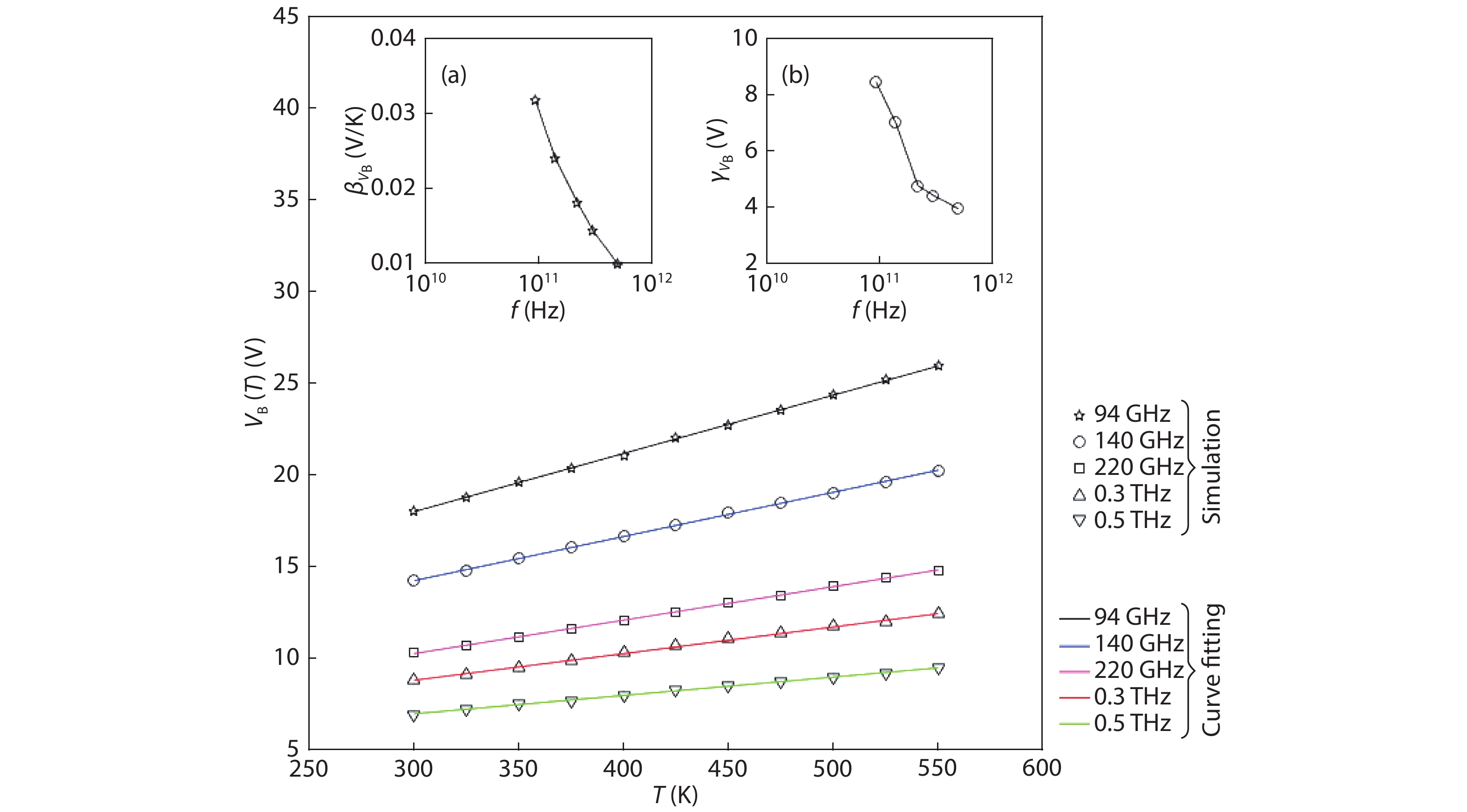
Fig. 1. (Color online) Variations of breakdown voltage of Si IMPATT sources operating at different mm-wave and THz frequencies with temperature; insets of the figure show (a) linear temperature coefficient of breakdown voltage, and (b) corresponding constant linear fitting parameter with operating frequency.

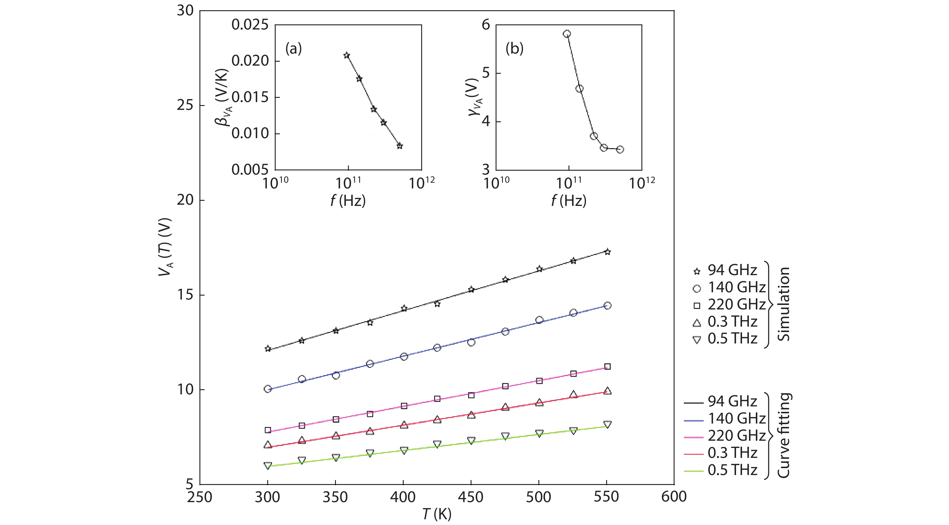
Fig. 2. (Color online) Variations of avalanche zone voltage drop of Si IMPATT sources operating at different mm-wave and THz frequencies with temperature; insets of the figure show (a) linear temperature coefficient of avalanche zone voltage drop and (b) corresponding constant linear fitting parameter with operating frequency.

Fig. 3. (Color online) Variations of avalanche zone width of Si IMPATT sources operating at different mm-wave and THz frequencies with temperature; insets of the figure show (a) linear temperature coefficient of avalanche zone width and (b) corresponding constant linear fitting parameter with operating frequency.

Fig. 4. (Color online) Variations of avalanche resonance frequency of Si IMPATT sources operating at different mm-wave and THz frequencies with temperature; insets of the figure show (a) quadratic temperature coefficient, (b) linear temperature coefficient of avalanche resonance frequency and (c) corresponding constant fitting parameter with operating frequency.

Fig. 5. (Color online) Variations of optimum frequency of Si IMPATT sources operating at different mm-wave and THz frequencies with temperature; the insets show (a) quadratic temperature coefficient, (b) linear temperature coefficient of optimum frequency and (c) corresponding constant fitting parameter with operating frequency.

Fig. 6. (Color online) Variations of peak negative conductance of Si IMPATT sources operating at different mm-wave and THz frequencies with temperature; insets of the figure show (a) quadratic temperature coefficient, (b) linear temperature coefficient of peak negative conductance and (c) corresponding constant fitting parameter with operating frequency.

Fig. 7. (Color online) Variations of susceptance corresponding to the peak negative conductance of Si IMPATT sources operating at different mm-wave and THz frequencies with temperature; insets of the figure show (a) quadratic temperature coefficient, (b) linear temperature coefficient of susceptance corresponding to the peak negative conductance and (c) corresponding constant fitting parameter with operating frequency.

Fig. 8. (Color online) Variations of RF power output of Si IMPATT sources operating at different mm-wave and THz frequencies with temperature; insets of the figure show (a) quadratic temperature coefficient, (b) linear temperature coefficient of RF power output and (c) corresponding constant fitting parameter with operating frequency.

Fig. 9. (Color online) Variations of DC to RF conversion efficiency of Si IMPATT sources operating at different mm-wave and THz frequencies with temperature; insets of the figure show (a) quadratic temperature coefficient, (b) linear temperature coefficient of DC to RF conversion efficiency and (c) corresponding constant fitting parameter with operating frequency.

Fig. 10. Variations of RF power output of Si IMPATT sources obtained from the large-signal simulation and experimental measurements^{[5, 18, 20]} at 500 K with operating frequency; inset shows the variations of DC to RF conversion efficiency of the sources obtained from the large-signal simulation and experimental measurement^[18] at 500 K with operating frequency.

Table 1. Optimized design parameters.

Table 2. Linear temperature coefficient and constant fitting parameter associated with DC parameters for the temperature range 300–550 K.

Table 3. Quadratic temperature coefficient, linear temperature coefficient and constant fitting parameter associated with large-signal parameters such as f_a, f_p and G_p for the temperature range of 300–550 K.

Table 4. Quadratic temperature coefficient, linear temperature coefficient and constant fitting parameter associated with large-signal parameters such as B_p, P_RF and η_L for the temperature range of 300–550 K.