• Advanced Photonics Nexus
  • Vol. 1, Issue 2, 026003 (2022)
Bing-Yan Wei1、2、†,*, Yuan Zhang3, Haozhe Xiong1、2, Sheng Liu1、2、*, Peng Li1、2, Dandan Wen1、2, and Jianlin Zhao1、2、*
Author Affiliations
  • 1Northwestern Polytechnical University, School of Physical Science and Technology, Shaanxi Key Laboratory of Optical Information Technology, Xi’an, China
  • 2Ministry of Industry and Information Technology, Key Laboratory of Light Field Manipulation and Information Acquisition, Xi’an, China
  • 3Chinese Flight Test Establishment, Xi’an, China
  • show less
    DOI: 10.1117/1.APN.1.2.026003 Cite this Article Set citation alerts
    Bing-Yan Wei, Yuan Zhang, Haozhe Xiong, Sheng Liu, Peng Li, Dandan Wen, Jianlin Zhao. Janus vortex beams realized via liquid crystal Pancharatnam–Berry phase elements[J]. Advanced Photonics Nexus, 2022, 1(2): 026003 Copy Citation Text show less
    (a) Radial cubic phase; (b) radial linear phase; (c) spiral phase with m=1; (d) superimposed phase structure of the former three; (f), (h) superimposed phase structures with the spiral phase of (e) m=2 and (g) m=6. The color variation from black to white represents the phase value from 0 to 2π, and it also indicates the optical axes varying from 0 to π when PB phase is introduced.
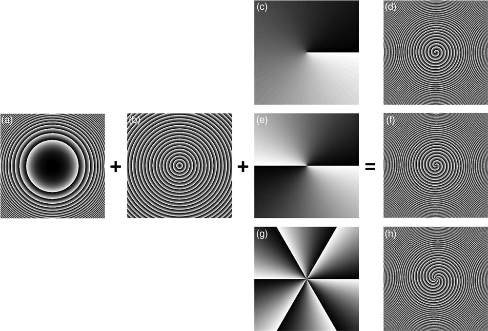
    Fig. 1. (a) Radial cubic phase; (b) radial linear phase; (c) spiral phase with m=1; (d) superimposed phase structure of the former three; (f), (h) superimposed phase structures with the spiral phase of (e) m=2 and (g) m=6. The color variation from black to white represents the phase value from 0 to 2π, and it also indicates the optical axes varying from 0 to π when PB phase is introduced.
    Micrographs of Janus-q-plate with (a) q=0.5, (b) q=1, and (c) q=3. The scale bar is 100 μm.
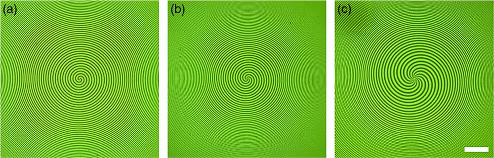
    Fig. 2. Micrographs of Janus-q-plate with (a) q=0.5, (b) q=1, and (c) q=3. The scale bar is 100  μm.
    Illustration of the Janus vortex beam (upper left) and optical setup for the generation and detection of Janus vortex beams. The red and black dashed lines represent the trajectories of the real part and the brought-into-real-space virtual part of the Janus vortex beam, respectively. The pairs of helical images are schematic diagrams of the opposite spiral phases of the Janus vortex beam.
    Fig. 3. Illustration of the Janus vortex beam (upper left) and optical setup for the generation and detection of Janus vortex beams. The red and black dashed lines represent the trajectories of the real part and the brought-into-real-space virtual part of the Janus vortex beam, respectively. The pairs of helical images are schematic diagrams of the opposite spiral phases of the Janus vortex beam.
    Propagation dynamics of Janus vortex beams with a Janus-q-plate of q=3. (a)–(i) Detected intensity distributions of the Janus vortex beams at z=9, 10, 12, 14, 15, 16, 18, 19, and 20 cm, respectively. The insets in (c)–(g) are zoom-in images of the central parts. (j) Experimental and theoretical propagation trajectories of the Janus vortex beam. The red circle marks the measured radius of the inner main ring, and the red and blue lines are parabolic fit and theoretical trajectory, respectively. Simulated side-view propagation of (k) Janus vortex beam and (l) autofocusing and autodefocusing circular Airy vortex beams.
    Fig. 4. Propagation dynamics of Janus vortex beams with a Janus-q-plate of q=3. (a)–(i) Detected intensity distributions of the Janus vortex beams at z=9, 10, 12, 14, 15, 16, 18, 19, and 20 cm, respectively. The insets in (c)–(g) are zoom-in images of the central parts. (j) Experimental and theoretical propagation trajectories of the Janus vortex beam. The red circle marks the measured radius of the inner main ring, and the red and blue lines are parabolic fit and theoretical trajectory, respectively. Simulated side-view propagation of (k) Janus vortex beam and (l) autofocusing and autodefocusing circular Airy vortex beams.
    (a)–(c) Simulated and (d)–(f) measured phase distributions of the Janus vortex beam at the first focal plane (first column), the FT plane of Lens 2 (second column), and the second focal plane (third column), respectively. The arrows in the lower right corners indicate the twist directions of the spiral phases.
    Fig. 5. (a)–(c) Simulated and (d)–(f) measured phase distributions of the Janus vortex beam at the first focal plane (first column), the FT plane of Lens 2 (second column), and the second focal plane (third column), respectively. The arrows in the lower right corners indicate the twist directions of the spiral phases.
    Simulated [(a), (d)] and experimental [(b), (e)] polarization distributions of the Janus vortex beam at the first/second focal plane. Red and green ellipses stand for the RCP and LCP states, respectively. (g) Simulated and (h) experimental intensity distributions at the FT plane of Lens 2 analyzed by a polarizer. The detected normalized Stokes parameter S3 distributions at these three planes are exhibited in (c), (f), and (i), respectively.
    Fig. 6. Simulated [(a), (d)] and experimental [(b), (e)] polarization distributions of the Janus vortex beam at the first/second focal plane. Red and green ellipses stand for the RCP and LCP states, respectively. (g) Simulated and (h) experimental intensity distributions at the FT plane of Lens 2 analyzed by a polarizer. The detected normalized Stokes parameter S3 distributions at these three planes are exhibited in (c), (f), and (i), respectively.
    Bing-Yan Wei, Yuan Zhang, Haozhe Xiong, Sheng Liu, Peng Li, Dandan Wen, Jianlin Zhao. Janus vortex beams realized via liquid crystal Pancharatnam–Berry phase elements[J]. Advanced Photonics Nexus, 2022, 1(2): 026003
    Download Citation