
Zhen-Zhe Lei, Yan-Jun Gu, Zhan Jin, Shingo Sato, Alexei Zhidkov, Alexandre Rondepierre, Kai Huang, Nobuhiko Nakanii, Izuru Daito, Masakai Kando, Tomonao Hosokai, "Supersonic gas jet stabilization in laser–plasma acceleration," High Power Laser Sci. Eng. 11, 06000e91 (2023)
- High Power Laser Science and Engineering
- Vol. 11, Issue 6, 06000e91 (2023)
Abstract
1 Introduction
Laser wakefield acceleration (LWFA) is attractive and promising to provide sources of radiation. It is expected to be a more compact facility compared with conventional accelerators[1,2]. A short pulse laser with ultra-high intensity (
Apart from delivering more accessible high-energy electron beams, LWFA is expected to have potential applications in tomography and bright X-ray sources in material sciences, as well as in radiation therapy and pharmacology. However, the stability of LWFA is still far away from that required for applications. Similar to vacuum accelerators, LWFA devices consist of the common injection and acceleration parts that can constitute a staging system. The injection and acceleration processes in plasma are essentially nonlinear. Both processes, driven by a laser pulse, depend nonlinearly on its characteristics as well as on the characteristics of the target plasma. Therefore, the investigation of the entire acceleration process is extremely complicated. Usually investigations of the injection and acceleration processes are focused on optimizing the final parameters of the electron bunches, such as the peak energy, beam charge, emittance and energy spread. For that purpose, the laser pulse parameters, such as the pulse intensity, duration and waist, as well as the gas target parameters, such as the gas density, density profiles and gas compounds, are carefully chosen to provide the required characteristics of electron beams.
However, optimizing the laser and target parameters cannot thoroughly solve the problem of stability and reproducibility in the LWFA process. Even with the fixed parameters one observes essential fluctuations by a factor of 2–3 of electron bunch energy, bunch charges, energy spreads and beam emittances. Moreover, the poor pointing stability of bunches sometimes transfers to beam decomposition. It is apparent that the study of the sources for such instabilities differs from that of parameter optimization.
Sign up for High Power Laser Science and Engineering TOC. Get the latest issue of High Power Laser Science and Engineering delivered right to you!Sign up now
Owing to the nonlinearity of the injection and acceleration processes, there are many parameters resulting in the plasma dynamics. Therefore, the best way of seeking the sources of instabilities is to extract the phenomena responsible for different stages, such as the formation of targets, laser pulse focusing and propagation, electron self-injection and acceleration. Target formation is the first stage of LWFA. To maintain the reproducibility of the accelerated electron beam, it requires a stable gas target in the vacuum chamber with a precise density distribution profile. It guarantees that the laser and plasma interact in a proper density region (
In this paper, we numerically and experimentally studied the instability originating from the gas jet due to the nonlinear fluid dynamics in the supersonic nozzle. In LWFA, supersonic nozzles are commonly used to provide spatially well-defined supersonic gas targets with a plateau density profile and sharp gas-vacuum boundaries. The design and application of supersonic nozzles have been proposed in many theoretical and experimental works[36–42]. Costa et al.[43] studied the behaviour of the gas outflow with the variations of nozzle throat narrowing via both simulations and experiments. Their results point out that having a supersonic gas flow out of the nozzle is a better way to be able to influence the flow density. Furthermore, the smoothing angle of the nozzle throat has an influence on the output flow density value.
2 Theories and simulations
When the high-velocity flow shear is combined with a confining nozzle wall, the corresponding velocities significantly decrease due to the boundary effect. Such boundary effect is not only a singularity of the flow field providing the seed of the vortex and turbulence, but also partially blocks the cross-section of the nozzle, resulting in significant variations of gas pressure. Therefore, the gas target becomes unstable and the laser focal position may exceed the allowable misalignment. According to fluid dynamics simulations, the density uncertainty perturbation in a simple-conical nozzle reaches more than
The fluid dynamics simulations are launched with ANSYS Fluent code, in which the Navier–Stokes equations are solved based on the finite volume method. To describe the turbulence, a shear-stress transport (SST)
A simple-conical nozzle is first examined here. The corresponding design and the numerical sketch are presented in Figures 1(a) and 1(b), respectively. The connection tube has a diameter of
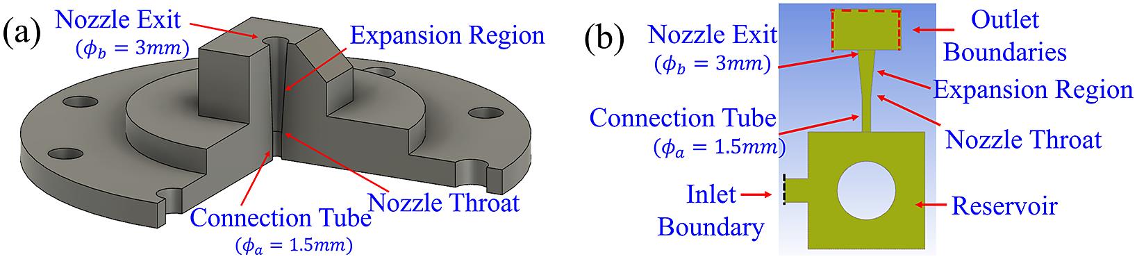
Figure 1.(a) Sketch of the simple-conical nozzle. (b) Schematic of the fluid dynamics simulation domains for the simple-conical nozzle.
The complicated mechanical structure of the solenoid valve is simplified by a circular obstacle inside the tank in the fluid dynamics simulations. In experiments, a high-speed solenoid valve from SMARTSHELL Co., Ltd. (Ref. A2-6443-FL-403713) is employed. It has a gas inlet with
The gas is pumped into the nozzle from the left-hand inlet (indicated by the black dashed line in Figure 1(b)) with the pressure input boundary condition, which is equivalent to that connected with a constant pressure reservoir. The initial pumping pressure is set to be a constant at
where
For an ideal isentropic nozzle with the exit size double that of the throat, the hydrogen flow becomes supersonic with the Mach number of
![]()
Figure 2.(a) Profiles of gas density, pressure and Mach number along the vertical direction from the connection tube to the exit. The density and pressure are normalized to the initial condition.
To generate the supersonic jet, the hydrogen gas is first pumped into the reservoir and then injected into the nozzle with the control of the solenoid valve. Due to the complicated structure of the reservoir and the valve motion, it is difficult to control the flow state from shot to shot during the pulse pumping. Figure 3(a) shows the velocity distribution of the gas flow with the streamlines (in black) in the reservoir. Vortex structures and eddies are clearly formed due to the interaction of the high-velocity flow and the static wall. Between the boundary walls and the central obstacle, there is a narrow steady flow with relatively high velocity. From the streamlines, one finds that the eddy regions have low flow velocities referring to local stagnation, which changes the pressure and the density distributions. The turbulent kinetic energy measured by the root mean square of the fluctuation in the flow velocity,
![]()
Figure 3.(a) Velocity distribution (normalized to the sound speed) and streamlines in the gas reservoir part. (b) Distribution of the turbulent kinetic energy in the gas reservoir part with a logarithmic scale. (c), (d) Velocity distributions and streamlines for the cases of left and down shift in the reservoir, respectively.
An initial perturbation is introduced into the fluid dynamics simulations to describe the stochastics of the valve motion. A group of simulations is launched by slightly shifting the central obstacle in the reservoir by 2 mm in the up, down, left and right directions, respectively. All of the other conditions are identical in these simulations. Two typical cases corresponding to the left-hand side and down-side shift are presented in Figures 3(c) and 3(d). The vortex distributions and the flow paths are significantly changed in these cases, as seen in Figures 3(a), 3(c) and 3(d). As a result, the gas flows being pumped into the nozzle are actually not identical under different conditions. In Figures 4(a) and 4(b), the gas density and pressure under different conditions are compared. The profiles are taken along the cross-section of the nozzle throat averaged within 0.5 mm in the vertical direction. The density perturbations reach 10%, while the density peak position shifts about 1 mm. For laser–plasma experiments, such as shock injections, the acceleration effect relies on the stability of the shock formation and the density downramp profile, which is very sensitive to the outflow angle and the Mach number of the gas jet.
![]()
Figure 4.(a) Gas density and (b) pressure profiles at the nozzle throat obtained in the different initial shift cases (black-none, red-up, blue-down, green-left, orange-right), respectively. The triangle marker directions refer to the shift directions of the central obstacle.
In order to stabilize the gas flow, a stilling chamber with a length of 20 mm and a diameter of
![]()
Figure 5.(a) Sketch of the converging–diverging nozzle. (b) Schematic of the fluid dynamics simulation domains for the converging–diverging nozzle. (c) Velocity distributions (normalized to the sound speed) and streamlines inside the stilling chamber part. The subplots from left to right correspond to the non-, up-, down-, left- and right-shift cases, respectively. (d) The density profiles in the converging region, diverging region and 1 mm above the exit are compared between the up-shift and down-shift cases.
3 Experimental results
The stabilization effect of the converging–diverging nozzle is also confirmed by the experimental measurement. We characterize our supersonic nozzles with a Mach–Zehnder interferometer method, as seen in Figure 6. A continuous-wave (CW) He-Ne laser (
![]()
Figure 6.Experimental schematic diagram of the Mach–Zehnder interferometer setup.
| S-C nozzle | C-D nozzle | |
|---|---|---|
| Std. (%) | 4.7/ | 1/ |
| Max. (%) | 13.5/ | 2.5/ |
Table 1. S-C nozzle and C-D nozzle represent the simple-conical nozzle and the converging–diverging nozzle, respectively. (Values not in bold are taken from the fluid dynamics simulations, while those in bold are obtained from the experimental measurements. Std. represents the standard deviation from 20 shots in the experiment and five cases in simulations. Max. represents the maximum discrepancy in the 20 shots in the experiment and five cases in simulations.)
To further confirm the stabilizing effect by adding the stilling chamber, the simple-conical nozzle and the converging–diverging nozzle are both tested in the LWFA experiments with the shock injection scheme[5,6], which were carried out with the Laser Acceleration Platform (LAPLACIAN) Ti:sapphire laser system (Amplitude Technologies) at RIKEN SPring-8 Center based on a chirped pulse amplification (CPA) technique. An ultra-short laser pulse (
![]()
Figure 7.Electron beam pointing distributions obtained in experiments with (a) the simple-conical nozzle and (b) the converging–diverging nozzle.
4 Conclusions
In summary, a method for generating stable and reproducible supersonic gas jets for laser–plasma interaction is proposed. The stilling chamber in a modified converging–diverging nozzle plays an important role in dissipating the nonlinear instabilities originated from the fluid boundary effects and the uncertainties of the solenoid valve pumping. Both the fluid dynamics simulations and the experimental measurements confirm that the density profiles of the converging–diverging nozzle have much lower perturbations than that of a simple-conical nozzle. In the LWFA experiments with a shock injection mechanism, the high electron pointing stability is obtained in the converging–diverging nozzle case. As such, the study proves the validity of the stilling chamber in stabilizing the gas jet, which will be useful and important to potential laser–plasma applications.
References
[1] T. Tajima, J. M. Dawson. Phys. Rev. Lett., 43, 267(1979).
[2] E. Esarey, C. B. Schroeder, W. P. Leemans. Rev. Mod. Phys, 81, 1229(2009).
[3] D. Umstadter, J. K. Kim, E. Dodd. Phys. Rev. Lett., 76, 2073(1996).
[4] T. Hosokai, M. Kando, H. Dewa, H. Kotaki, S. Kondo, N. Hasegawa, K. Nakajima, K. Horioka. Opt. Lett., 25, 10(2000).
[5] P. Tomassini, M. Galimberti, A. Giulietti, D. Giulietti, L. A. Gizzi, L. Labate, F. Pegoraro. Phys. Rev. Spec. Top. Accel. Beams, 6, 121301(2003).
[6] H. Suk, N. Barov, J. B. Rosenzweig, E. Esarey. Phys. Rev. Lett., 86, 1011(2001).
[7] J. Faure, C. Rechatin, A. Norlin, A. Lifschitz, Y. Glinec, V. Malka. Nature, 444, 737(2006).
[8] W. P. Leemans, B. Nagler, A. J. Gonsalves, C. Tóth, K. Nakamura, C. G. R. Geddes, E. Esarey, C. B. Schroeder, S. M. Hooker. Nat. Phys., 2, 696(2006).
[9] T. Hosokai, K. Kinoshita, A. Zhidkov, A. Maekawa, A. Yamazaki, M. Uesaka. Phys. Rev. Lett., 97, 075004(2006).
[10] X. Davoine, E. Lefebvre, C. Rechatin, J. Faure, V. Malka. Phys. Rev. Lett., 102, 065001(2009).
[11] M. Chen, E. Esareya, C. B. Schroeder, C. G. R. Geddes, W. P. Leemans. Phys. Plasmas, 19, 033101(2012).
[12] R. Lehe, A. F. Lifschitz, X. Davoine, C. Thaury, V. Malka. Phys. Rev. Lett., 111, 085005(2013).
[13] S. Corde, C. Thaury, A. Lifschitz, G. Lambert, K. T. Phuoc, X. Davoine, R. Lehe, D. Douillet, A. Rousse, V. Malka. Nat. Commun., 4, 1501(2013).
[14] A. Buck, J. Wenz, J. Xu, K. Khrennikov, K. Schmid, M. Heigoldt, J. M. Mikhailova, M. Geissler, B. Shen, F. Krausz, S. Karsch, L. Veisz. Phys. Rev. Lett., 110, 185006(2013).
[15] F. Li, J. F. Hua, X. L. Xu, C. J. Zhang, L. X. Yan, Y. C. Du, W. H. Huang, H. B. Chen, C. X. Tang, W. Lu, C. Joshi, W. B. Mori, Y. Q. Gu. Phys. Rev. Lett., 111, 015003(2013).
[16] N. Bourgeois, J. Cowley, S. M. Hooker. Phys. Rev. Lett., 111, 155004(2013).
[17] M. Zeng, M. Chen, L. L. Yu, W. B. Mori, Z. M. Sheng, B. Hidding, D. A. Jaroszynski, J. Zhang. Phys. Rev. Lett., 114, 084801(2015).
[18] M. P. Tooley, B. Ersfeld, S. R. Yoffe, A. Noble, E. Brunetti, Z. M. Sheng, M. R. Islam, D. A. Jaroszynski. Phys. Rev. Lett., 119, 044801(2017).
[19] Z. Jin, H. Nakamura, N. Pathak, Y. Sakai, A. Zhidkov, K. Sueda, R. Kodama, T. Hosokai. Sci. Rep., 9, 20045(2019).
[20] D. N. Gupta, S. R. Yoffe, A. Jain, B. Ersfeld, D. A. Jaroszynski. Sci. Rep., 12, 20368(2022).
[21] K. V. Grafenstein, F. M. Foerster, F. Haberstroh, D. Campbell, F. Irshad, F. C. Salgado, G. Schilling, E. Travac, N. Weiße, M. Zepf, A. Döpp, S. Karsch. Sci. Rep., 13, 11680(2023).
[22] J. Faure, Y. Glinec, A. Pukhov, S. Kiselev, S. Gordienko, E. Lefebvre, J. P. Rousseau, F. Burgy, V. Malka. Nature, 431, 541(2004).
[23] S. P. D. Mangles, C. D. Murphy, Z. Najmudin, A. G. R. Thomas, J. L. Collier, A. E. Dangor, E. J. Divall, P. S. Foster, J. G. Gallacher, C. J. Hooker, D. A. Jaroszynski, A. J. Langley, W. B. Mori, P. A. Norreys, F. S. Tsung, R. Viskup, B. R. Walton, K. Krushelnick. Nature, 431(2004).
[24] C. G. R. Geddes, C. Toth, J. van Tilborg, E. Esarey, C. B. Schroeder, D. Bruhwiler, C. Nieter, J. Cary, W. P. Leemans. Nature, 431, 538(2004).
[25] I. Blumenfeld, C. E. Clayton, F. J. Decker, M. J. Hogan, C. K. Huang, R. Ischebeck, R. Iverson, C. Joshi, T. Katsouleas, N. Kirby, W. Lu, K. A. Marsh, W. B. Mori, P. Muggli, E. Oz, R. H. Siemann, D. Walz, M. M. Zhou. Nature, 445, 741(2007).
[26] S. Kneip, C. McGuffey, J. L. Martins, S. F. Martins, C. Bellei, V. Chvykov, F. Dollar, R. Fonseca, C. Huntington, G. Kalintchenko, A. Maksimchuk, S. P. D. Mangles, T. Matsuoka, S. R. Nagel, C. A. J. Palmer, J. Schreiber, K. T. Phuoc, A. G. R. Thomas, V. Yanovsky, L. O. Silva, K. Krushelnick, Z. Najmudin. Nat. Phys., 6, 980(2010).
[27] K. T. Phuoc, S. Corde, C. Thaury, V. Malka, A. Tafzi, J. P. Goddet, R. C. Shah, S. Sebban, A. Rousse. Nat. Photonics, 6, 308(2012).
[28] N. D. Powers, I. Ghebregziabher, G. Golovin, C. Liu, S. Chen, S. Banerjee, J. Zhang, D. P. Umstadter. Nat. Photonics, 8, 28(2014).
[29] M. Litos, E. Adli, W. An, C. I. Clarke, C. E. Clayton, S. Corde, J. P. Delahaye, R. J. England, A. S. Fisher, J. Frederico, S. Gessner, S. Z. Green, M. J. Hogan, C. Joshi, W. Lu, K. A. Marsh, W. B. Mori, P. Muggli, N. Vafaei-Najafabadi, D. Walz, G. White, Z. Wu, V. Yakimenko, G. Yocky. Nature, 515, 92(2014).
[30] E. Adli, A. Ahuja, O. Apsimon, R. Apsimon, A.-M. Bachmann, D. Barrientos, F. Batsch, J. Bauche, V. K. Berglyd Olsen, M. Bernardini, T. Bohl, C. Bracco, F. Braunmüller, G. Burt, B. Buttenschön, A. Caldwell, M. Cascella, J. Chappell, E. Chevallay, M. Chung, D. Cooke, H. Damerau, L. Deacon, L. H. Deubner, A. Dexter, S. Doebert, J. Farmer, V. N. Fedosseev, R. Fiorito, R. A. Fonseca, F. Friebel, L. Garolfi, S. Gessner, I. Gorgisyan, A. A. Gorn, E. Granados, O. Grulke, E. Gschwendtner, J. Hansen, A. Helm, J. R. Henderson, M. Hüther, M. Ibison, L. Jensen, S. Jolly, F. Keeble, S.-Y. Kim, F. Kraus, Y. Li, S. Liu, N. Lopes, K. V. Lotov, L. Maricalva Brun, M. Martyanov, S. Mazzoni, D. Medina Godoy, V. A. Minakov, J. Mitchell, J. C. Molendijk, J. T. Moody, M. Moreira, P. Muggli, E. Öz, C. Pasquino, A. Pardons, F. Peña Asmus, K. Pepitone, A. Perera, A. Petrenko, S. Pitman, A. Pukhov, S. Rey, K. Rieger, H. Ruhl, J. S. Schmidt, I. A. Shalimova, P. Sherwood, L. O. Silva, L. Soby, A. P. Sosedkin, R. Speroni, R. I. Spitsyn, P. V. Tuev, M. Turner, F. Velotti, L. Verra, V. A. Verzilov, J. Vieira, C. P. Welsch, B. Williamson, M. Wing, B. Woolley, G. Xia. Nature, 561(2018).
[31] W. T. Wang, K. Feng, L. Ke, C. Yu, Y. Xu, R. Qi, Y. Chen, Z. Qin, Z. Zhang, M. Fang, J. Liu, K. Jiang, H. Wang, C. Wang, X. Yang, F. Wu, Y. Leng, J.-S. Liu, R. Li, Z. Xu. Nature, 595, 516(2021).
[32] W. P. Leemans, A. J. Gonsalves, H.-S. Mao, K. Nakamura, C. Benedetti, C. B. Schroeder, C. Tóth, J. Daniels, D. E. Mittelberger, S. S. Bulanov, J.-L. Vay, C. G. R. Geddes, E. Esarey. Phys. Rev. Lett., 113, 245002(2014).
[33] A. J. Gonsalves, K. Nakamura, J. Daniels, C. Benedetti, C. Pieronek, T. C. H. de Raadt, S. Steinke, J. H. Bin, S. S. Bulanov, J. van Tilborg, C. G. R. Geddes, C. B. Schroeder, C. Tóth, E. Esarey, K. Swanson, L. Fan-Chiang, G. Bagdasarov, N. Bobrova, V. Gasilov, G. Korn, P. Sasorov, W. P. Leemans. Phys. Rev. Lett., 122, 084801(2019).
[34] A. Döpp, C. Thaury, E. Guillaume, F. Massimo, A. Lifschitz, I. Andriyash, J. P. Goddet, A. Tazfi, K. T. Phuoc, V. Malka. Phys. Rev. Lett., 121, 074802(2018).
[35] L. T. Ke, K. Feng, W. T. Wang, Z. Y. Qin, C. H. Yu, Y. Wu, Y. Chen, R. Qi, Z. J. Zhang, Y. Xu, X. J. Yang, Y. X. Leng, J. S. Liu, R. X. Li, Z. Z. Xu. Phys. Rev. Lett., 126, 214801(2021).
[36] S. Semushin, V. Malka. Rev. Sci. Instrum., 72, 2961(2001).
[37] K. Schmid, L. Veisz. Rev. Sci. Instrum., 83, 053304(2012).
[38] S. Lorenz, G. Grittani, E. Chacon-Golcher, C. M. Lazzarini, J. Limpouch, F. Nawaz, M. Nevrkla, L. Vilanova, T. Levato. Matter Radiat. Extremes, 4, 015401(2019).
[39] L. Rovige, J. Huijts, A. Vernier, I. Andriyash, F. Sylla, V. Tomkus, V. Girdauskas, G. Raciukaitis, J. Dudutis, V. Stankevic, P. Gecys, J. Faure. Rev. Sci. Instrum., 92, 083302(2021).
[40] C. Aniculaesei, H. T. Kim, B. J. Yoo, K. H. Oh, C. H. Nam. Rev. Sci. Instrum., 89, 025110(2018).
[41] H. Xu, G. Chen, D. Patel, Y. Cao, L. Ren, H. Xu, H. Shao, J. He, D. E. Kim. AIP Adv., 11, 075313(2021).
[42] O. Zhou, H.-E. Tsai, T. M. Ostermayr, L. Fan-Chiang, J. Tilborg, C. B. Schroeder, E. Esarey, C. G. R. Geddes. Phys. Plasmas, 28, 093107(2021).
[43] G. Costa, M. P. Anania, A. Biagioni, F. G. Bisesto, M. Del Franco, M. Galletti, M. Ferrario, R. Pompili, S. Romeo, A. R. Rossi, A. Zigler, A. Cianchi. JINST, 17, C01049(2022).
[44] F. Brandi, F. Giammanco. Opt. Express, 19, 25479(2011).
[45] J. Couperus, A. Köhler, T. A. W. Wolterink, A. Jochmann, O. Zarini, H. M. J. Bastiaens, K. J. Boller, A. Irman, U. Schramm. Nucl. Instrum. Methods Phys. Res. Sect. A, 830, 504(2016).
[46] A. Adelmann, B. Hermann, R. Ischebeck, M. C. Kaluza, U. Locans, N. Sauerwein, R. Tarkeshian. Appl. Sci., 8, 443(2018).
[47] F. R. Menter. AIAA J., 32, 1598(1994).
[48] J. D. Anderson. Fundamentals of Aerodynamics(2010).
[49] Z. Lei, Z. Jin, A. Zhidkov, N. Pathak, Y. Mizuta, K. Huang, N. Nakanii, I. Daito, M. Kando, T. Hosokai. Prog. Theor. Exp. Phys., 2023, 033J01(2023).


Set citation alerts for the article
Please enter your email address

© Copyright 2018-2021 | Chinese Laser Press. All Rights Reserved 沪ICP备15018463号-20