
Shijie Liu, Chunlai Li, Rui Xu, Guoliang Tang, Jianyu Wang. Hyperspectral Imaging System Using Electronic Multi-Slot Combination Coding[J]. Acta Optica Sinica, 2020, 40(1): 0111026
- Acta Optica Sinica
- Vol. 40, Issue 1, 0111026 (2020)
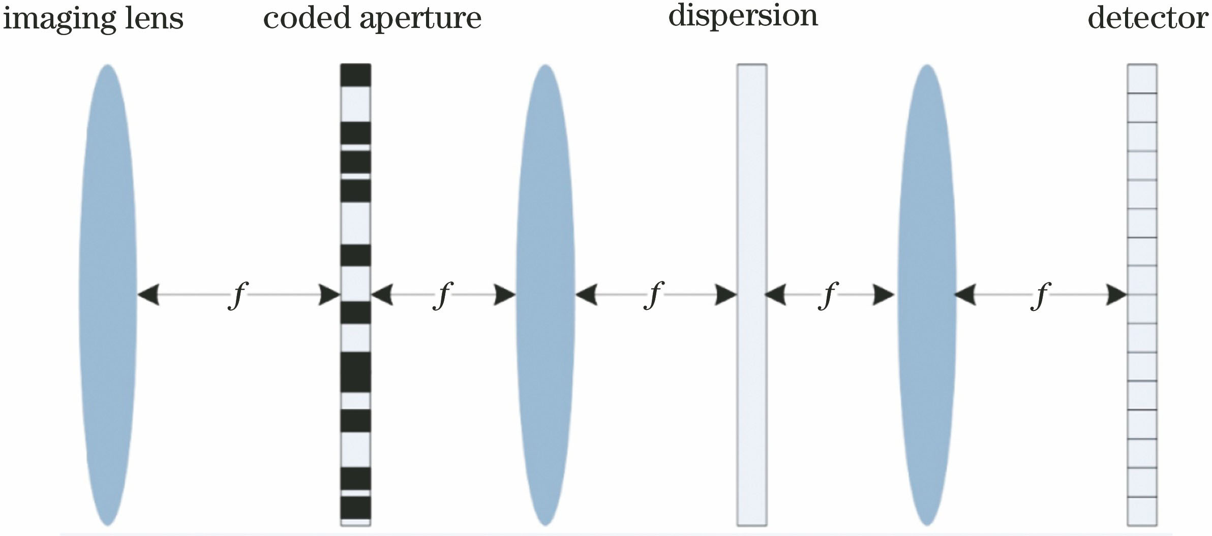
Fig. 1. SD-CASSI system
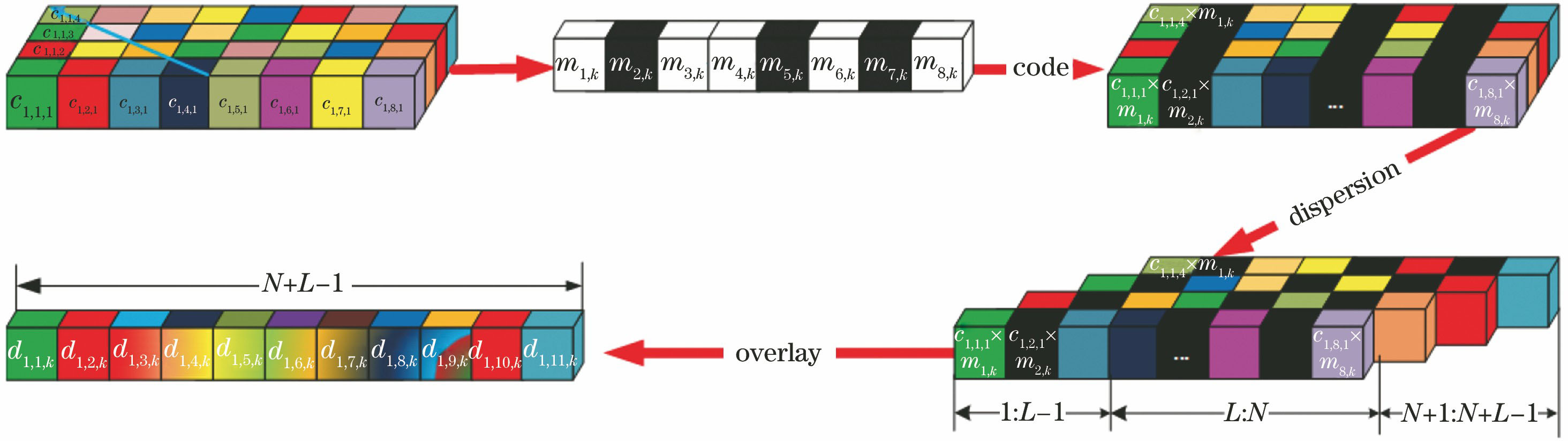
Fig. 2. Data flow of the kth row measurement
Fig. 3. Comparison of two-dimensional random coding and multi-slot combination coding. (a) Two-dimensional random coding; (b) multi-slot combination coding
Fig. 4. Correspondence between the measured matrix and measured vector
Fig. 5. Coded sampling results and recovery results with different sampling rates. (a) Original image; (b) traditional sampling data; (c) coded sampling data; (d) 20% sampling recovery; (e) 50% sampling recovery; (f) 80% sampling recovery
Fig. 6. Comparison of spectral recovery results at different sampling rates
Fig. 7. Evaluation of recovery results for different sampling rates. (a) pSNR for spatial information recovery; (b) SCF for spectral information recovery
Fig. 8. Electronic multi-slot combined encoding hyperspectral imaging system based on liquid crystal light valve
Fig. 9. Imaging target and sampling results used in experiment. (a) Imaging target; (b) sampling results
Fig. 10. Recovery results of experiments with different sampling rates. (a) 20%; (b) 50%; (c) 80%
Fig. 11. Spectral recovery results at different positions. (a) Position 1 and position 2; (b) position 3 and position 4
Fig. 12. Recovery results under different sampling rates in outdoor experiments. (a) Data cube recovered at 80% sampling rate; (b) recovery result of spectral curve at position A under different sampling rates
Fig. 13. Calibration under different fields of view
| ||||||||||||||||||||||||||||||||||||||||||||||||||||||||||||||
Table 1. Digital simulation results of different algorithms under different sample rates

Set citation alerts for the article
Please enter your email address
© Copyright 2018-2021 | Chinese Laser Press. All Rights Reserved 沪ICP备15018463号-20