2,000,000 fps 2D and 3D imaging of periodic or reproducible scenes with single-pixel detectors

Wenjie Jiang; Yongkai Yin; Junpeng Jiao; Xian Zhao; Baoqing Sun

doi:10.1364/PRJ.461064

Abstract

Single-pixel imaging (SPI) can capture 2D images of the target with only a nonpixelated detector, showing promising application potential in nonvisible spectral imaging, low-photon imaging, lidar, and other extreme imaging fields. However, the imaging mechanism of traditional SPI makes it difficult to achieve high imaging speed, which is a primary barrier for its widespread application. To address this issue, in this work, we propose and demonstrate a novel high-speed 2D and 3D imaging scheme based on traditional SPI, termed time-resolved single-pixel imaging (TRSPI). Previous SPI works mainly utilize correlation between a stable target and iterative illumination masks to reconstruct a single image. In TRSPI, by further exploiting correlation information between a dynamic scene and every static mask, we can reconstruct a series of time-varying images of the dynamic scene, given the dynamic scene is repetitive or reproducible. Experimentally, we conducted 2D and 3D imaging on a rotating chopper with a speed of 4800 revolutions per minute (rpm), and imaging speeds up to 2,000,000 fps. It is believed that this technology not only opens up a novel application direction for SPI, but also will provide a powerful solution for high-speed imaging.

1. INTRODUCTION

We live in a dynamic world, where all matter is in a vibrant state. Some dynamic events occur in a microsecond, nanosecond, or even faster time scale, in which the human eye or common digital cameras cannot observe and record the instantaneous picture of these scenes. Being able to observe and analyze these dynamic processes is undoubtedly critical for scientific discoveries and technical innovations. To do this, some professional high-speed focal plane array (FPA) cameras have been developed that can capture images at a speed of up to millions of frames per second (fps) [1]. Nevertheless, this imaging speed is already close to the physical limit of the FPA detector, making it difficult to continue to be improved significantly. To further overcome hardware speed barriers, some computational high-speed imaging schemes have been presented, which can surpass the imaging speed extremum of FPA cameras in the form of camera array [2,3], compressive sensing [4,5], and spectral encoding [6,7]. Despite all these achievements, we should realize that the apparatus complexity and financial expensiveness have largely prohibited the application of high-speed imaging. To develop a proper technology with both technique and financial affordability, even for a specific application, is therefore highly desirable.

In this work, we propose and demonstrate a high-speed imaging scheme based on single-pixel imaging (SPI), called time-resolved single-pixel imaging (TRSPI). SPI is a correlation imaging method that retrieves images based on structured illumination and nonpixelated detection. The prototype of SPI can be traced back to Hadamard transform optics in the 1970s [8]. In the last two decades, there has been a surge of investigation on SPI, largely inspired by the development of ghost imaging [9,10], compressive sensing [11,12], and for its potential application at special wavelengths [13 –15]. However, there is one inescapable fact: SPI usually requires a large number of structured illuminations during the capture of a single image. As a result, SPI can only be implemented for static targets or relatively low frame rate photography. In order to enable SPI to work at a video frame rate or even faster, various methods based on algorithms or hardware have been proposed, such as deep-learning-based SPI [16], Fourier SPI [17], cross-frame correlation [18], and high-speed lighting arrays [19,20]. However, all these works are implemented and limited with pattern and signal one-to-one acquisition mode, so that the imaging speed of SPI is still determined by the refresh rate of the spatial light modulation (SLM).

In traditional SPI, correlation between a stable target and iterative illumination masks is mainly utilized, rendering it a time-consuming approach. In our proposed TRSPI, by further exploiting correlation information between a dynamic scene and every static mask, we are able to design a high-speed imaging technology, given the dynamic scene is repetitive or reproducible. In TRSPI, the imaging frame rate is no longer limited by the refresh rate of SLM, but only depends on the working bandwidth and sampling rate of a single-pixel detection module. In previous works, a similar idea has been proposed by implementing ultrashort pulse laser for illumination and as a highly precise synchronization timer. Combining with the high response speed of a single-pixel detector, one can perform fluorescence lifetime imaging [21,22] and non-line-of-sight imaging [23]. In our work, we develop TRSPI in a more general scenario, with no request on the ultrashort pulse laser. We demonstrate that TRSPI can be conducted with ambient light illumination and apply it for 2D and 3D imaging of high-speed rotating targets, thereby achieving significant improvement in image quality and pixel scale. In addition, compared to multipixel FPA cameras, a single-pixel detector has lower cost, higher sensitivity, and higher bandwidth, so our TRSPI scheme will be a better choice for high-speed imaging of repetitive or reproducible varying scenes.

Sign up for Photonics Research TOC. Get the latest issue of Photonics Research delivered right to you！Sign up now

2. METHODS

A. SPI

Normal camera technology uses FPA to capture spatial information pixel by pixel simultaneously, whereas in SPI, as detectors are nonpixelated, the role of spatial sampling is shifted to the illumination end. A series of 2D structured illuminations are iteratively projected over the target area. If we vectorize every illumination structure into a row vector, then the spatial sampling process of SPI can be expressed as $Y = A X,$ (1)where $A = [a_{m p}]$ is an $M \times P$ matrix that denotes the sampling basis, and each row represents a vectorized 2D illumination structure. $X = [x_{p}]$ represents the object, and $Y = [y_{m}]$ is the single-pixel signal. Therefore $X$ and $Y$ are column vectors with a dimension of $P$ and $M$ , respectively. While $P$ corresponds to the pixel number of scene defined by the illumination, $M$ is the total number of measurements. Then Eq. (1) can be written in detail as $y_{m} = \sum_{p = 1}^{P} a_{m p} \cdot x_{p} .$ (2)

Specifically, $A$ is usually a binary matrix composed of 0 and 1, which can be implemented experimentally by using SLM like a digital micromirror device (DMD). In some situations, if differential measurement is implemented, then $A$ could be a matrix containing $- 1$ and 1. In this case, each row vector of $A$ corresponds to a pair of illumination patterns that are opposite to each other. An advantage of differential measurement is to suppress the low-frequency component of noise [24].

Once single-pixel signals are acquired, an image can be obtained computationally by exploiting the correlation between these signals and their corresponding illumination basis $A$ , which is essential to solve an inverse problem. Mostly, two types of reconstruction approaches are used: iterative correlation algorithms and compressive sensing algorithms. For iterative correlation algorithms, a widely used illumination basis is the Hadamard basis for its maximum sampling efficiency. The iterative reconstruction process can be expressed as $\hat{X} = A Y .$ (3)

Here $\hat{X}$ is the estimation of $X$ , and $A$ stands for a Hadamard matrix. Equation (3) is the inverse process of Eq. (1), given the fact that the inverse of a Hadamard matrix equals itself.

Alternatively, compressive sensing can solve the inverse of Eq. (1) from sub-Nyquist acquisition $(M ≪ P)$ by exploiting the sparsity of natural images, which has been well studied in SPI. The reconstruction function can be represented as $\hat{X} = \arg \min_{X} \frac{1}{2} {‖ Y - A X ‖}_{2}^{2} + λ Ψ (X),$ (4)where $Ψ (X)$ is regularization term that represents the sparseness constraint of $X$ . $λ$ is the penalty parameter to balance the residuals and sparsity in the optimization process.

B. TRSPI

According to the imaging principle of normal SPI above, the imaging speed of SPI is generally slow, which makes it impossible to image scenes that vary rapidly in the time domain. Here, we propose a novel SPI scheme, namely, TRSPI, which is extremely suitable for high-speed varying periodic or reproducible dynamic scenes. The schematic diagram of TRSPI is shown in Fig. 1. The target is at a high speed, but repetitive motion can be measured many times. During each period, illumination with a certain structure is employed, under which a single-pixel detector samples fast to obtain time-resolved detections. 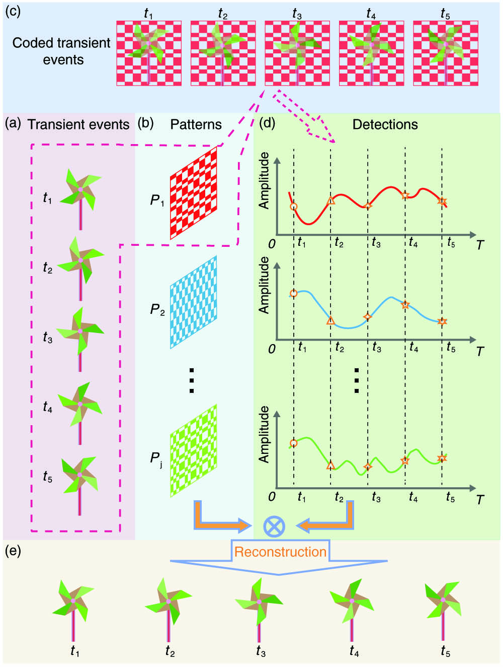Digitization with a certain sampling rate determines how many moments (the number of $t_{i}$ ) are resolved. In the next period, the same measurement process is repeated under a different illumination mask. The concise mathematical expression of TRSPI’s imaging acquisition process can still be shown in Eq. (1). Note that $X$ is no longer a column vector that only represents the spatial information of a scene, but a $P \times T$ 2D matrix carrying spatial and temporal information of a dynamic scene. $Y$ will also be an $M \times T$ 2D matrix representing $M$ detection signal sequences of length $T$ . Thus, the acquisition process of TRSPI can be expressed in detail as $y_{m t} = \sum_{p = 1}^{P} a_{m p} \cdot x_{p t} .$ (5)

Figure 1.Schematic diagram of TRSPI. (a) Transient events at different instants are indicated as $t_{i}$ . (b) Different illumination patterns $P_{j}$ ; (c) coded transient event in one period under a certain illumination pattern; (d) under each illumination pattern, a single-pixel detection histogram is measured. By applying different illumination patterns over repetitive events, a series of pattern-encoded histograms are obtained. (e) By extracting signals at the same $t_{i}$ from different histograms, a reconstruction at that instant can be achieved.

As the motion of an object is periodic, the object at the same moment in different periods should be in the exactly same position. This means, if we extract the detection signal at the same moment from different periods, a reconstruction of the object at this position can be conducted. In this way, the image at time $t_{i}$ contained in the entire period $T$ can be reconstructed accordingly, whether using an iterative correlation algorithm or a compressive sensing algorithm. Their reconstruction process can be expressed as $\hat{X} (t_{i}) = A Y (t_{i}),$ (6)and $\hat{X} (t_{i}) = \arg \min_{X (t_{i})} \frac{1}{2} {‖ Y (t_{i}) - A X (t_{i}) ‖}_{2}^{2} + λ Ψ [X (t_{i})] .$ (7)

C. TRSPI for 3D Imaging Based on Fourier Transform Profilometry

3D imaging has a wide range of applications in precision manufacturing, automatic navigation, digital archiving of cultural heritage, surgical guidance, etc. However, current 3D imaging technology also suffers from huge challenges in capturing high-speed varying dynamic scenes. To solve this, we develop TRSPI for time-resolved spatial 3D imaging by combining existing static 3D imaging techniques. One of the commonly used 3D imaging techniques is Fourier transform profilometry (FTP) [25]. As shown in Fig. 2(a), the hardware configuration of classic FTP consists of fringe projection and image recording. The projection branch, consisting of an LED light source, condenser lens, grating, and camera lens 2, projects a standard fringe pattern onto the surface of the object. The standard fringe pattern will be modulated by the shape of object, which will be recorded as a deformed fringe image via the imaging branch consisting of the camera lens 1 and a CMOS chip. Then, 3D topography of the object is recovered using a reconstruction algorithm from the deformed fringe image. According to the Helmholtz reciprocity, as shown in Fig. 2(b), FTP technology has been verified to be able to run in the SPI system [26,27]. Logically, we also introduce the FTP technique on the proposed TRSPI to achieve time-resolved 3D imaging.

Figure 2.Classic and reciprocal SPI configurations of FTP. (a) Classic configuration of the conventional FTP; (b) according to the Helmholtz reciprocity, a grating is added into SPI configuration for 3D imaging based on FTP theory. (c) The principle of height calculation with the phase difference between the surface of the object and the reference plane.

The 3D reconstruction principle of FTP in an SPI system is consistent with the classic FTP. In the 3D SPI system based on FTP, a 2D line grating is added to the image plane of a collecting lens. The grating generates a standard fringe pattern, described as $I_{0} (x, y) = a_{0} + b_{0} \cos [φ_{0} (x, y)] .$ (8)

Here $a_{0}$ is the background intensity and $b_{0}$ the modulation intensity, which are both constant for the whole pattern. $φ_{0} (x, y)$ is the initial phase distribution corresponding to the reference plane, whose height is set to zero. When an object is measured, the standard fringe pattern will be modulated by the surface of the object. The background and modulation intensities will no longer be constant due to the surface texture and nonuniform reflectivity of the object. More importantly, the phase distribution will be changed according to the shape of the object. Therefore, the deformed fringe pattern can be described as $I_{d} (x, y) = a (x, y) + b (x, y) \cos [φ (x, y)] .$ (9)

This deformed fringe pattern is recorded by a CMOS camera in conventional FTP or by the SPI system based on FTP. The recorded image can be used to retrieve the phase distribution $φ (x, y)$ and then to reconstruct the shape of the object. According to Euler’s formula, Eq. (9) can be rewritten as $I_{d} (x, y) = a (x, y) + \frac{b (x, y)}{2} [e^{i φ (x, y)} + e^{- i φ (x, y)}] .$ (10)

In order to obtain the frequency spectrum of the fundamental component $e^{i φ (x, y)}$ , a Fourier transform is performed first on the deformed fringe image, and then a proper bandpass filter is used to select the positive first-order component of the Fourier spectrum. Complex spatial distribution of the fundamental component can be solved by the inverse Fourier transform, which can be described as follows: $I_{f} (x, y) = \frac{b (x, y)}{2} e^{i φ (x, y)} .$ (11)

Here we ignore the spectrum aliasing and assume that the positive first-order component can be extracted exactly with a suitable bandpass filter. Then the phase distribution can be retrieved by the following calculation: $φ (x, y) = \arctan {\frac{Im [I_{f} {x, y}]}{Re [I_{f} {x, y}]}} .$ (12)

Here Im and Re denote the imaginary and real parts of a complex value, respectively. As shown in Fig. 2(c), $φ (x, y)$ is modulated by the shape of the object; by formulating the modulation with the proper system model, the height of the object can be calculated by the phase difference between the deformed fringe image and the standard fringe pattern. The calculation process is as follows: $h (x, y) = S [φ (x, y) - φ_{0} (x, y)] = S [Δ φ (x, y)] .$ (13)

Here $S$ denotes the function of the system model. It should be noted that the value range of the arc tangent function leads to wrapped phase distribution between $- π$ and $π$ ; thus, the spatial phase unwrapping algorithm is required before calculating the phase difference.

3. EXPERIMENTS AND ANALYSIS

A. Experimental Setup

To demonstrate the feasibility of the proposed TRSPI scheme, 2D and 3D imaging experiments were built, respectively, as shown in Fig. 3. The complete 2D imaging experiment configuration is illustrated in Fig. 3(a), which can be divided into two modules, including active structural illumination and signal detection. In the active structural illumination module, a collimated LED source together with a reflecting mirror is used to uniformly illuminate the DMD (ViALUX, V-7001), and then the camera lens is employed to project patterns loaded on the DMD onto the target area. The signal detection module of 2D imaging consists of a single-pixel detector and a data acquisition (DAQ) module, which is used to detect reflected light from objects. Moreover, DMD can release a trigger signal to the DAQ whenever the pattern is refreshed, which is used to accurately ensure the synchronization between structured illumination and signal detection. The experimental configuration of 3D imaging is not different from 2D imaging, except for the signal detection module. The experimental configuration of the signal detection module for 3D imaging is shown in Fig. 3(b). A camera lens is used to collect the reflected light from the target, and then a beam splitter (BS) bisects the beam passing through the camera lens. One of them keeps the same propagation direction and passes through the grating and lens 1 to be detected by detector 1; the other one changes the original propagation direction and passes through lens 2 to be detected by detector 2. The grating is binarized and placed at a position slightly offset from the image plane of the camera lens to achieve sinusoidal modulation. During the imaging process, detector 1 and detector 2 record data synchronously, and these two sets of data are used to reconstruct a striped image and a uniform image, respectively. These two images are then used together to recover a high-quality 3D shape of the target.

Figure 3.Experimental setup of TRSPI for 2D and 3D imaging. (a) Complete TRSPI experimental configuration for 2D imaging; (b) detection module of TRSPI for 3D imaging.

B. Digital Calibration

In the detection process, a set of patterns is continuously projected to encode the dynamic scene, with the additional requirement that the exposure time of each pattern is equal to the period of the dynamic scene. For most situations, we do not know how long the period of these dynamic scenes is. Therefore, before imaging, we need to measure the period of the dynamic scene. It can be achieved using constructed TRSPI configurations above. First, we use the active structural illumination module of the TRSPI system to project a regular stationary pattern, as shown in Fig. 4(a), onto the target area. Then, a single-pixel detector continuously detects for a certain period to record, which is much longer than the period of the dynamic scene. The recorded signal has obvious periodic fluctuation, as shown in Fig. 4(b), from which we can obtain the exact duration of one period of the dynamic scene. The refresh rate of DMD is then set based on this time.

Figure 4.Measure period of a dynamic scene and digital calibration. (a) Regular checkerboard pattern loaded on the DMD when measuring the period of the dynamic scene; (b) continuous signal recorded by a single-pixel detector when the scene is illuminated by pattern (a), whose length exceeds a period of the dynamic scene. The red dashed box represents the time length of one period of the dynamic scene. (c) Digital calibration scheme when there is a slight mismatch between the period of the dynamic scene and exposure time of each illumination pattern.

Ideally, the exposure time of each pattern and the period of the dynamic scene are exactly the same, and under the synchronization of triggers released by the DMD, the signals of different periods recorded by DAQ are synchronized in time. However, the highest accuracy of DMD exposure time is at the microsecond level, which may result in submicrosecond deviations between the exposure time of each pattern and the period of dynamic scene. More than that, these deviations are accumulated during the imaging process, causing the recorded signals of different periods to be misaligned in time, which will seriously affect the reconstruction quality. To solve this problem, we propose a digital calibration scheme. Take one of the possible scenarios as an example, when the exposure time of DMD is slightly longer than the period of dynamic scene; the recorded signal sequence under each pattern is shown in Fig. 4(c). It can be seen that the tail of each signal contains the signal of the next encoding pattern. We clipped the heads and tails of these signals, as shown by the red dashed line in Fig. 4(c). In this way, the processed signals are aligned in time; then they are grouped according to different moments. Finally, the instantaneous images of the scene at the corresponding moments are, respectively, reconstructed. Of course, the proposed digital alignment method is applicable whether the exposure time of the DMD is slightly longer or slightly shorter than the scene period.

C. 2D TRSPI Experiment

Using the above experimental configuration and calibration scheme, we first completed the time-resolved 2D SPI experiment. The imaging target is a rapidly rotating chopper at a speed of 4800 revolutions per minute (rpm), meaning it has an angular velocity of $160 π rad / s$ and a maximum linear velocity of about 25 m/s. To make rotation details of the chopper more noticeable, distinct numbers and letters are painted on the chopper plate. In the experiment, to maximize the sampling and reconstruction efficiency, we choose compressive sensing as our reconstruction algorithm. Specifically, TVAL3 was employed as our reconstruction algorithm [28]. TVAL3 utilizes the property of image sparsity in the gradient transform domain to conduct compressive calculation. Total variation is adopted as the regularization term for sparse constraint. 21,000 random binary patterns with 1 and $- 1$ distribution are used as our encoding matrix. In actual operation, it is implemented in a differential means by 42,000 patterns with 0 and 1 distribution. The exposure time of each pattern is set to be the same as the rotation period of the chopper, i.e., 12,500 ms, resulting in a total image acquisition time of 8.75 min. Each pattern in a resolution of $256 \times 256 pixels$ is generated using a middle area of DMD in $768 \times 768 pixels$ , i.e., each pattern pixel is formed by merging $3 \times 3$ adjacent DMD pixels. Here, we define the full sampling ratio as 65,536 ( $256 \times 256$ ) spatial encoding and detections. Correspondingly, 21,000 spatial encoding and detections stand for a 32% sampling ratio. In the signal detection module, the single-pixel detector (PDA100A2) has a working bandwidth of 90 kHz at a gain of 40 dB, and the DAQ (NI-6366) digitizes signals at a sampling rate of 2 MS/s. As a result, our TRSPI is capable of imaging at 2,000,000 fps in non-real time. In one rotation period of the chopper, 25,000 instantaneous images can be reconstructed. Figure 5 shows part of the imaging results—12 selected instantaneous images with an interval of 1 ms. As can be seen from the imaging results, our scheme has excellent imaging capability both in the space domain and in the time domain.

Figure 5.Selected 12 instantaneous frames from 2D TRSPI results (see Visualization 1 for more details).

D. 3D TRSPI Experiment

In the second experiment, we completed the time-resolved 3D imaging and evaluated the accuracy of the imaging results. The imaging target is a high-speed rotating 3D fan at a speed of 4800 rpm. This fan is 3D printed by us so that we can accurately digitize its 3D shape for reconstructed image analysis. In our 3D imaging experiment, the inverse Hadamard transform is used as the reconstruction algorithm instead of the compressed sensing algorithm, because with the addition of a 2D line grating in the imaging light path, the scene is no longer sparse in some transform domains and it is difficult to use compressive sampling. Since two single-pixel detectors are used in the signal detection module, two images of the scene can be reconstructed simultaneously, one with deformed fringes, as shown in Fig. 6(a), and the other is uniform, as shown in Fig. 6(b). Both images have a spatial resolution of $128 \times 128 pixels$ , and the total imaging time for differential measurement is nearly 7 min. Generally, the Fourier spectrum of the deformed fringe image commonly has a zeroth-order component of large magnitude and wide range, which leads to spectrum aliasing when filtering the positive first-order component. Hence, the uniform image is used to normalize the background of the deformed fringe image [29]. As shown in Fig. 6(c), the zeroth-order component in the Fourier spectrum is dramatically suppressed after the background normalization; thus we can better select the positive first-order component with a Hann window, as shown in Fig. 6(d). Then the wrapped phase can be retrieved from the inverse Fourier transform of the selected positive first-order component, as shown in Fig. 6(e). The 2D Goldstein branch cut phase unwrapping algorithm is employed for phase unwrapping [30]. Finally, the shape of the dynamic object can be reconstructed with a calibrated system model, as shown in Fig. 6(f).

Figure 6.3D TRSPI process based on FTP. (a) One reconstructed frame from detector 1; (b) reconstructed frame from detector 2 at the same time as in (a); (c) Fourier spectrum of (a) after background normalization; (d) positive first-order component of (c), selected with a Hann window; (e) wrapped phase obtained by inverse Fourier transform of (d); (f) reconstructed 3D shape corresponding to current frame (see Visualization 2 for more details). (g) Evaluation of the measurement uncertainty.

To make a simple demonstration of 3D reconstruction, we just assume that the system model describing the phase-to-height conversion can be approximated with a polynomial expression. We empirically select the third-order polynomial as the model function. The calibration of the system model is essentially a least-squares estimation of the polynomial coefficients. A white plate perpendicular to the optical axis of the illumination camera lens serves as the height gauge. The plate at the initial position is defined as the reference plane, and then it is moved to nine positions (corresponding to nine different heights), along with the optical axis, and the height shift is 4 mm between two adjacent positions. Therefore, nine groups of phase differences and their corresponding heights are obtained, which can be used to fit the model function pixel by pixel. We compare the deviation between the measured point cloud and the computer-aided design (CAD) model of the fan to evaluate the accuracy of 3D imaging. First, the point cloud is aligned to the CAD model with rigid transformation, and then the cloud-to-mesh (C2M) distances according to each 3D point in the point cloud are calculated, as shown in Fig. 6(g). The root mean square error (RMSE) of the C2M signed distances is 0.279 mm. Considering the height range of system calibration is $4 \times 9 = 36 mm$ , we can claim that our system has a relative uncertainty of $\pm 1.5 %$ ( $0.279 \times 1.96 / 36$ ) for 3D measurement at the 95% confidence level.

4. DISCUSSION AND CONCLUSION

In summary, we propose and demonstrate a high-speed 2D and 3D imaging approach using single-pixel detections, which achieves imaging speeds up to 2,000,000 fps. As we well know, imaging speed, or time resolution, has always been a drawback of SPI. In the conventional SPI mode, dynamic masks are always used to continuously encode a stable object, which results in the SPI frame rate being limited by the refresh rate and the number of masks. As a result, even with the use of state-of-the-art SLM to refresh dynamic masks and advanced algorithms to reduce the number of masks, the imaging speed of SPI is usually only a few tens of frames per second. However, in our proposed TRSPI, encoding is done by exploiting the relative motion between the dynamic scenes and each static mask, so that the encoding speed is determined by the motion speed of the dynamic scenes. In this way, the frame rate of TRSPI is no longer limited by the SLM refresh rate, but only depends on the working bandwidth and sampling rate of the single-pixel detection module. Single-pixel detectors tend to have a very high working bandwidth; thus TRSPI will offer a qualitative improvement in imaging speed compared to conventional SPI. In addition, compared with other existing high-speed cameras based on array detectors, single-pixel detectors are always easier and less expensive to manufacture with high speed and sensitivity. With not only these advantages, the simplicity of a single-pixel detector also makes it easy to be combined with other technologies, such as spectrometry and interferometry. With the combination of these technologies, TRSPI is expected to achieve high-speed hyperspectral imaging and phase imaging.

Many transient phenomena are not observed, not because they are unimportant, but because a high-speed camera is normally too expensive. Although the requirement for repetitive measurement restricts the application of TRSPI to some extent, it is undoubtedly that there are many high-speed repetitive scenes, and photographing these scenes has important research and application value. Examples include inspecting high-speed rotating or oscillating components in various instruments, analyzing the 3D deformation of rigid components caused by high-speed motion, studying some reproducible chemical reaction processes, analyzing the composition of materials based on laser-induced plasma, and even understanding ultrafast laser and related photonics technology. In a word, we believe our TRSPI approach will have great applications in various areas.

References

[1] Y. Kondo, K. Takubo, H. Tominaga, R. Hirose, N. Tokuoka, Y. Kawaguchi, Y. Takaie, A. Ozaki, S. Nakaya, F. Yano, T. Daigen. Development of ‘HyperVision HPV-X’ high-speed video camera. Shimadzu Rev., 69, 285-291(2012).

[2] B. Wilburn, N. Joshi, V. Vaish, E.-V. Talvala, E. Antunez, A. Barth, A. Adams, M. Horowitz, M. Levoy. High performance imaging using large camera arrays. ACM Trans. Graph., 24, 765-776(2005).

[3] A. Agrawal, M. Gupta, A. Veeraraghavan, S. G. Narasimhan. Optimal coded sampling for temporal super-resolution. IEEE Computer Society Conference on Computer Vision and Pattern Recognition, 599-606(2010).

[4] L. Gao, J. Liang, C. Li, L. V. Wang. Single-shot compressed ultrafast photography at one hundred billion frames per second. Nature, 516, 74-77(2014).

[5] Y. Liu, X. Yuan, J. Suo, D. J. Brady, Q. Dai. Rank minimization for snapshot compressive imaging. IEEE Trans. Pattern Anal. Mach. Intell., 41, 2990-3006(2018).

[6] K. Goda, K. Tsia, B. Jalali. Serial time-encoded amplified imaging for real-time observation of fast dynamic phenomena. Nature, 458, 1145-1149(2009).

[7] K. Nakagawa, A. Iwasaki, Y. Oishi, R. Horisaki, A. Tsukamoto, A. Nakamura, K. Hirosawa, H. Liao, T. Ushida, K. Goda, F. Kannari. Sequentially timed all-optical mapping photography (STAMP). Nat. Photonics, 8, 695-700(2014).

[8] J. Decker. Hadamard–transform image scanning. Appl. Opt., 9, 1392-1395(1970).

[9] T. B. Pittman, Y. Shih, D. Strekalov, A. V. Sergienko. Optical imaging by means of two-photon quantum entanglement. Phys. Rev. A, 52, R3429-R3432(1995).

[10] J. H. Shapiro. Computational ghost imaging. Phys. Rev. A, 78, 061802(2008).

[11] R. G. Baraniuk. Compressive sensing [lecture notes]. IEEE Signal Process. Mag., 24, 118-121(2007).

[12] J. Romberg. Imaging via compressive sampling. IEEE Signal Process. Mag., 25, 14-20(2008).

[13] A.-X. Zhang, Y.-H. He, L.-A. Wu, L.-M. Chen, B.-B. Wang. Tabletop X-ray ghost imaging with ultra-low radiation. Optica, 5, 374-377(2018).

[14] G. M. Gibson, B. Sun, M. P. Edgar, D. B. Phillips, N. Hempler, G. T. Maker, G. P. Malcolm, M. J. Padgett. Real-time imaging of methane gas leaks using a single-pixel camera. Opt. Express, 25, 2998-3005(2017).

[15] R. I. Stantchev, X. Yu, T. Blu, E. Pickwell-MacPherson. Real-time terahertz imaging with a single-pixel detector. Nat. Commun., 11, 2535(2020).

[16] M. Lyu, W. Wang, H. Wang, H. Wang, G. Li, N. Chen, G. Situ. Deep-learning-based ghost imaging. Sci. Rep., 7, 17865(2017).

[17] Z. Zhang, X. Ma, J. Zhong. Single-pixel imaging by means of Fourier spectrum acquisition. Nat. Commun., 6, 6225(2015).

[18] S. Sun, J.-H. Gu, H.-Z. Lin, L. Jiang, W.-T. Liu. Gradual ghost imaging of moving objects by tracking based on cross correlation. Opt. Lett., 44, 5594-5597(2019).

[19] Z.-H. Xu, W. Chen, J. Penuelas, M. Padgett, M.-J. Sun. 1000 fps computational ghost imaging using LED-based structured illumination. Opt. Express, 26, 2427-2434(2018).

[20] W. Zhao, H. Chen, Y. Yuan, H. Zheng, J. Liu, Z. Xu, Y. Zhou. Ultrahigh-speed color imaging with single-pixel detectors at low light level. Phys. Rev. Appl., 12, 034049(2019).

[21] Q. Pian, R. Yao, N. Sinsuebphon, X. Intes. Compressive hyperspectral time-resolved wide-field fluorescence lifetime imaging. Nat. Photonics, 11, 411-414(2017).

[22] F. Rousset, N. Ducros, F. Peyrin, G. Valentini, C. D’Andrea, A. Farina. Time-resolved multispectral imaging based on an adaptive single-pixel camera. Opt. Express, 26, 10550-10558(2018).

[23] G. Musarra, A. Lyons, E. Conca, Y. Altmann, F. Villa, F. Zappa, M. J. Padgett, D. Faccio. Non-line-of-sight three-dimensional imaging with a single-pixel camera. Phys. Rev. Appl., 12, 011002(2019).

[24] B. Sun, M. Edgar, R. Bowman, L. Vittert, S. Welsh, A. Bowman, M. Padgett. Differential computational ghost imaging. Computational Optical Sensing and Imaging, CTu1C-4(2013).

[25] M. Takeda, K. Mutoh. Fourier transform profilometry for the automatic measurement of 3-D object shapes. Appl. Opt., 22, 3977-3982(1983).

[26] Z. Zhang, J. Zhong. Three-dimensional single-pixel imaging with far fewer measurements than effective image pixels. Opt. Lett., 41, 2497-2500(2016).

[27] Y. Ma, Y. Yin, S. Jiang, X. Li, F. Huang, B. Sun. Single pixel 3D imaging with phase-shifting fringe projection. Opt. Laser Eng., 140, 106532(2021).

[28] C. Li. An efficient algorithm for total variation regularization with applications to the single pixel camera and compressive sensing(2010).

[29] C. Zuo, T. Tao, S. Feng, L. Huang, A. Asundi, Q. Chen. Micro Fourier transform profilometry (μftp): 3D shape measurement at 10,000 frames per second. Opt. Laser Eng., 102, 70-91(2018).

[30] R. M. Goldstein, H. A. Zebker, C. L. Werner. Satellite radar interferometry: two-dimensional phase unwrapping. Radio Sci., 23, 713-720(1988).