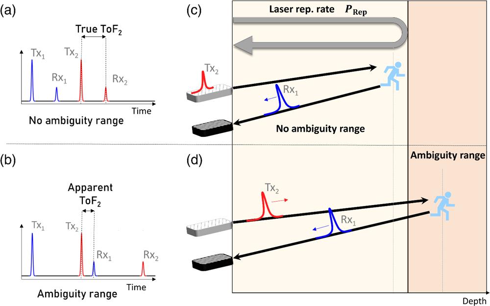
Fig. 1. Ambiguity range origin illustrated by the emission of two pulses (Tx₁ and Tx₂) and their respective reception on the detector (Rx₁ and Rx₂). (a), (c) When the target is located within the ambiguity range, each received pulse comes back to the detector before the next one is emitted; hence, the ToF is correctly recovered. (b), (d) In the ambiguity range case, the distance of the target is beyond the distance associated to the laser repetition rate, such that the first received pulse Rx₁ can be detected after the second transmitted pulse Tx₂ is emitted. In this case, the origin of Rx₁ might be wrongfully attributed to Tx₂, skewing the ToF measurement.

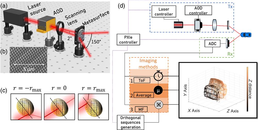
Fig. 2. Architecture of the ultrafast high FoV metasurface lidar. (a) Emission and scanning modules of the lidar. Our lidar consists of a high repetition rate 633 nm laser coupled to a 2D AOD operating as a narrow angle scanning module with a limited FoV of 2deg×2deg, but capable of reaching scanning speeds at the megahertz beam repointing frequency. The low FoV of the AOD is further enhanced by cascading a metasurface acting as an FoV expander, allowing the device to reach 150 deg FoV in both horizontal and vertical directions. The beam impinges on the metasurface after being focused into a 100μm spot by a scanning lens. (b) Scanning electron microscopy image of the metasurface sample. (c) Metasurface functionality concept. The metasurface is designed as a gradually varying beam deflector. The output angle varies as a function of position of the impact point of the AOD deflected beam on the metasurface. The large angle beam deflecting functionality of the metasurface is obtained by choosing, for example here, a parabolic phase profile. (d) Lidar imaging scheme. The proposed lidar works on a bistatic configuration. A PXIe controller is driving and synchronizing the emission, scanning, and detection modules. The detector is an MPPC, allowing detection with high sensitivity, necessary at the working wavelength of 633 nm due to the high level of background noise and atmospheric absorption. Three imaging methods are tested and compared, namely, the single-pulse ToF, averaged multiple pulses ToF and CDMA. AOD, acousto-optic deflector; ADC, analog-to-digital converter; MF, matched filter; Tx, transmission channel; and Rx: reception channel.

Fig. 3. d-ToF imaging schemes and demonstration. (a) S-pulse d-ToF recovery scheme for four pixels. The peak detection method relies on finding the maximum of the derivative of the received signal (black dot in inset) in each time gated slice, indicated by blue, green, red, and magenta colors. ToF is measured in each time-gated slice by measuring the time between the start trigger (green triangle), initiated at the time when the pulse is sent by the transmission channel (Tx) and the stop trigger (red square), stopped when the pulse is received by the reception channel (Rx). Each pulse corresponds to a different scanned position on the FoV or pixel. (b) M-pulse d-ToF recovery scheme for two pixels. The peak detection method is the same as in S-pulse, but instead of considering only one pulse per pixel, multiple laser pulses are sent to the same pixel and ToF values are averaged. The desired effect is to increase the SNR, but this also reduces the ambiguity range. In this example, n=2 pulses are averaged on each pixel. (c) ToF imaging raster scanning scheme. Each pixel corresponds to one or multiple pulses depending on the use of S-pulse or M-pulse method. (d) Experimental setup for the comparison of the imaging capacities of the different d-ToF techniques. Two objects, object 1 (square and circle) and object 2 (one square), are placed in the FoV of the lidar at 1.5 and 3.4 m, respectively. (e), (f) 3D point clouds obtained with the S-pulse and M-pulse techniques, respectively, at the same scanning speed of 1.8 MHz. (e) The scene is imaged using S-pulse ToF, with an ambiguity range of 80 m. (f) The two targets appear at the correct distance but experience low resolution and SNR due to the low intensity of the returned signal. This problem is mitigated by sending m=27 pulses at the same position and averaging the results. However, this approach creates ambiguity on the object 2 position, resulting in ghost imaging artifact for any object located beyond the ambiguity range of 3 m. Indeed, the object 1 is within the ambiguity range and appears at the right distance. Instead, the object 2 unreliably appears at a much shorter apparent ToF, corresponding to a depth of 0.4 m. S-pulse, single pulse and M-pulse, averaged multiple pulses.

Fig. 4. Block CDMA architecture and imaging. (a) CDMA ToF recovery scheme for three pixels. Instead of sending a single pulse or a sequence of pulses separated by the same duration to achieve M-pulse ToF measurement, we propose instead to send a specific pulse sequence at each pixel. The collection of sequences has to satisfy an orthogonality condition in order to ensure an optimal ToF recovery. The latter is performed using a matched filter, built on the correlation of the received signal with the different emitted sequences. The ToF is obtained by finding the time delay corresponding to the autocorrelation peak. The three outputs of the matched filter are computed in postprocessing and displayed on the Xcorri plots, with the corresponding ToF associated with each object present on the scene on the left. (b) Several encoding patterns can be considered; we present here only a comparison between two orthogonal sequence generation techniques. In blue, the OOC and in red, the PSs. The length of one sequence of PS quickly exceeds the one of OOC when going toward larger sequence family cardinalities, thus increasing the duration of the PS sequences, which further increases the ambiguity ranges. (c) CDMA raster scanning scheme. The scanning is performed by pixel blocks (here three pixels per CDMA block) without idle listening time between each block, i.e., a new sequence is immediately emitted on the following pixel block without waiting for a listening time [the example in (a) shows three pixels only]. As a generalization of this methodology, we consider that a block (blue boxes) corresponds to a collection of M orthogonal sequences sent one after another. When the whole block of pixels is emitted, the lidar sends the same orthogonal sequence collection for the next block again. In this scheme, the ambiguity range is no longer related to the idle listening time but is now defined by the time elapsed between the emission of two identical sequences from two consecutive blocks. (d) Imaging demonstration using the CDMA scheme with 14 OOC pulse sequences. This technique images the target at the correct distance thanks to its extended ambiguity range of 1155 m. However, when the returned data are input in the matched filter without further treatment, a wrong distance is computed on the edges of the targets due to the difference of returned intensity on the edge of the object. (e) This blooming artifact is suppressed using hard limiting filter, which clips the data at a given threshold in order to ignore the high-amplitude difference of returned signal. Xcorr, cross-correlation; CDMA, code division multiple access; and M, cardinality of the sequence family.

Fig. 5. (a) Imaging speed improvement enabled by the use of the CDMA technique with OOC codes. The theoretical repetition rate of the S-pulse technique as a function of the ambiguity distance is computed and compared to the one of CDMA for different block sizes; hence, the ambiguity ranges. Laser modulation speed is 200 MHz. As predicted, the CDMA offers a speed improvement to the system, from a factor 3 to a factor 35 as compared to the S-pulse. At our experimental scanning speed of 1.8 MHz, using OOC CDMA theoretically extends the ambiguity range from 80 m with S-pulse to 1155 m. Three regions corresponding to the speed capabilities of our lidar prototype are highlighted: in green, the region where the scanning is stable; in blue, the region where the scanning speed reaches the limits of the AOD; and in red, the inaccessible region. The zoomed inset shows that our lidar is almost meeting the requirements of the automotive lidar, with an ambiguity range of 234 m at a scanning speed of 4 MHz. For an image with a typical resolution for automotive lidars, this corresponds to a frame rate of 20 fps. (b) Highly reflective USAF-1951 calibration target used for the resolution measurement. The red line represents the position of the vertical cut for the resolution visualization. (c) Measurement of resolvable sizes for different scanning speeds with the S-pulse technique. As the scanning speed increases, the image suffers from a resolution loss, essentially due to the 1D distortion along the direction of the fast axis scanning of the AOD. The asymmetric beam shape after the AOD results in the blurring of a vertical cut of a USAF-1951 calibration target as displayed in (d). Insets represent the measured reflectivity of the lidar imaging of a USAF-1951 target located at 3 m distance, using two different beam repointing speeds of 750 kHz (bottom) and 5 MHz (top). (d) Spatial Fourier transform of the lidar image of a resolution measurement USAF-1951 target. This measurement exhibits with clear boundaries the origin of the three regions shown in (a). Color scale represents the normalized amplitude of the Fourier transform.

Fig. 6. (a) SNR comparison for the different imaging techniques as a function of the emission power. SNR is controlled by sending less signal on the scene. (b) Capacity to operate in low SNR environment. ToF of a single point is retrieved and averaged over N = 10,000 times for different emission powers. Decreasing the emission power is equivalent to performing imaging in a lower SNR environment. We consider that the operation of the lidar is correct if the standard deviation of the N = 10,000 distance measurements is low enough (error bars). The results show that M-pulse is more resilient to SNR conditions, followed by the CDMA with hard limiter. (c) Flowchart of the SNR measurement process in our setup. We assume that the internal noise of the detector is negligible as compared to the external illumination noise, and that this noise is constant throughout the measurement, as the setup is placed in a controlled low-light environment. This is statistical and relies on measurements of points corresponding to emission of a single pulse, 27 equal-space pulses, or one sequence of pulses from a family of 14 OOC codes, for S-pulse, M-pulse, or CDMA, respectively. The amplitude of the detected desired signal is obtained by averaging N times the detected pulse amplitudes. In the M-pulse case, the amplitude of one point corresponds to the average value of the 27 pulses of this point. In the CDMA case, the amplitude of one point corresponds to the average value of the amplitudes of the three pulses of the OOC sequence. The last step represented in dotted line corresponds to the measurement presented in (b).

Fig. 7. Metasurface fabrication: (a) GaN metasurface process steps and (b) SEM image of the metasurface.

Table 1. PS family for p=5.

Table 2. Strict OOC family with M=5.