
Emil Marinov, Renato Juliano Martins, Mohamed Aziz Ben Youssef, Christina Kyrou, Pierre-Marie Coulon, Patrice Genevet. Overcoming the limitations of 3D sensors with wide field of view metasurface-enhanced scanning lidar[J]. Advanced Photonics, 2023, 5(4): 046005
- Advanced Photonics
- Vol. 5, Issue 4, 046005 (2023)
Abstract
1 Introduction
The unveiling of the laser range finder,1 in which a directional light pulse is backscattered by a reflective object toward a detector, has enabled new imaging technology currently known as “pulsed laser scanning lidar.” This technique uses direct time-of-flight (d-ToF) measurements to calculate the depth at which the reflective object is positioned by recording the elapsed time separating emission and detection of a single laser pulse (S-pulse). Sequentially repeating the d-ToF measurement, for example, by scanning two angles, provides 1D depth information over a 2D field of view (FoV), thus achieving tridimensional imaging. The depth distance of each scanned point is given by , where is the speed of light. Although S-pulse d-ToF is remarkable in terms of simplicity of architecture, it suffers from a low signal-to-noise ratio (SNR) and poor accuracy at longer distances. Furthermore, this technique implies a trade-off between the maximum measurable distance, namely, ambiguity range () and the pulse repetition rate (), given by . The trade-off follows the expression:
Going beyond these basic limitations and further increasing the performance and compactness of current scanning lidar systems requires: (i) enlarging the FoV with high angular resolution, (ii) extending the actual imaging depth by reducing the SNR, (iii) achieving flexible scanning to any desired regions of interest and multiple illuminations, and (iv) improving beam repointing speed. Several solutions have been proposed recently to address one or several of these challenges. Among them, solid-state and compact lidar systems relying on phased array antennas,2,3 and active metasurfaces4,5 are currently emerging as the most suitable candidates. Both solutions propose to operate near and/or below the subwavelength phase addressing regime, a necessary condition to further increase the FoV, but which results in extremely dense and complex driving electronics. By combining simple active beam-steering systems with passive beam-shaping devices, for example, by cascading an acousto-optic deflector (AOD) with a phase-gradient metasurface,6 it is possible to drastically reduce the driving electronics complexity down to only two voltage channels,7 while achieving extreme FoVs, megahertz beam repointing, and multizone simultaneous imaging performance. Here we further extend the depth-imaging capabilities of such metasurface-enhanced lidar systems by proposing a new scanning methodology that resolves the problem of ambiguity range associated with this imaging lidar technique.
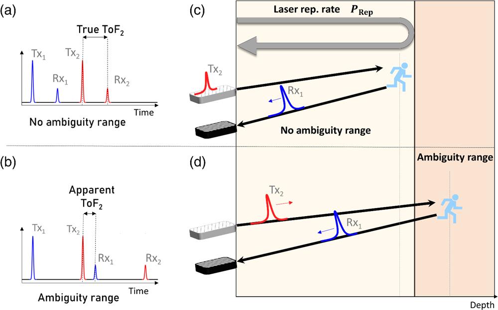
To better understand the trade-off between the ambiguity range () and the pulse repetition rate, in Fig. 1, we illustrate the two regimes, namely, unambiguous (top) and ambiguous regimes (bottom), by displaying two transmitted pulses, and and their backscattered counterparts received on the detectors and . When the target depth is lower than the ambiguity range [Figs. 1(a) and 1(c)], the origin of the returned pulse is unambiguous, as it is detected before a subsequent pulse is emitted. In the unambiguous regime, the ToF can be retrieved without ambiguity on the object’s distance. In comparison, in Figs. 1(b) and 1(d), a pulse propagating on a longer distance and returning after the emission of a second pulse results in an ambiguity on the true temporal origin of the pulse. The latter case is defined as a “second time around echo”8 and corresponds to “an echo received after a time delay exceeding one pulse-repetition interval but less than two pulse-repetition intervals.” This same principle is used to define the “third time around echo,” and more generally the multiple time around echo, with the parameter , corresponding to the number of integer times of contained in the true distance of a target. Accordingly, the true range of a target can be expressed as
Sign up for Advanced Photonics TOC. Get the latest issue of Advanced Photonics delivered right to you!Sign up now
![]()
Figure 1.Ambiguity range origin illustrated by the emission of two pulses (Tx1 and Tx2) and their respective reception on the detector (Rx1 and Rx2). (a), (c) When the target is located within the ambiguity range, each received pulse comes back to the detector before the next one is emitted; hence, the ToF is correctly recovered. (b), (d) In the ambiguity range case, the distance of the target is beyond the distance associated to the laser repetition rate, such that the first received pulse Rx1 can be detected after the second transmitted pulse Tx2 is emitted. In this case, the origin of Rx1 might be wrongfully attributed to Tx2, skewing the ToF measurement.
For automotive lidar application, a critical requirement is performing fast beam repointing between two consecutive imaging points to enable 3D imaging at very high speed, for example, to sense fast moving targets, or to increase the number of pixels to detect small objects over a large FoV. Typically, the desired imaging refreshing rate is 30 fps (frames per second) with each frame containing at least .9 This translates to a scanning speed of around 6 MHz, which corresponds to a 50 m ambiguity range for single-pulse ToF and does not meet the requirement of 200 m range for forward-looking automotive lidars.9
Mitigation strategies have been developed to handle both SNR and ambiguity range issues. As for the ability of the system to operate in lower SNR environments, one factor of interest is the performance of the receiving module. Early works in atmospheric lidars have shown that the use of spectral10
However, the ambiguity range issue can also be alleviated in several ways. Multiplexing pairs of source–detector with each covering a different angular region effectively increases the pulse density without decreasing the ambiguity range. The first 3D real-time lidar created by Velodyne in 2005 already exploited this idea by multiplexing 64 pairs of sources and detectors.21 The same strategy can be obtained by multiplexing different wavelengths as done in Baraja lidars.22 However, while these two strategies have been subjected to research,23 they have the drawback of higher complexity, impacting the reliability and the cost of the device, thus limiting their use in high-volume industries.
Resolving the ambiguity range issue has been a concern since the development of radar technology. A basic method used to resolve the ambiguity on the distance measurement is based on a priori assumptions about the correct depth of a target.24 Although this method might have some practical interest in topographic airborne lidars where ground-truth topographic maps already exist, it is impractical in most lidars, since their prime goal is to determine an unknown distance. Another approach is the jittering technique,25 which relies on the fact that the apparent ToF of a pulse returning from a target located further than [Figs. 1(b) and 1(d)] is dependent on the . Indeed, a slightly different results in a difference in and hence changes the retrieved ToF. Conversely, the ToF of pulses coming back from a range within is not impacted by a slight change in . Therefore, by slightly alternating the of the emitted pulses, it is possible to discriminate targets within from targets beyond the . Additionally, by measuring the change in the apparent ToF when jittering the , one can deduce the multiple times around echo in Eq. (2) and thus the true range of the target. Such method has been implemented and optimized26 for airborne lidar application, but it relies on imaging blocks of around 10 consecutive frames26 of the same scene with different to solve the range ambiguity. This considerably slows down the frame rate and might have limited practical interest for automotive lidars. Analogously, multiple have been used to extend the ambiguity range in single-photon lidar systems,27
More advanced techniques, such as interpulse30 or intrapulse31 coding, are state-of-the-art of ambiguity range resolution in radar. Both techniques result in effectively increasing , the latter by modulating the frequency of emitted pulses, i.e., sending chirps and implementing a matched filter on the output, and the former by modulating the whole pulse train with a specific modulation scheme. So far, these were considered for radar and have yet not been implemented for lidar application. However, some of the presented concepts were reused in lidar,32 where the authors modulated the emitted single pulse with a random generated sequence and recovered the ToF by correlating the received signal with this generated sequence. The same matched filter principle was later implemented multiple times, mainly in theoretical works,33,34 with the additional requirement that the modulation sequences have optimal correlation properties.35 In this scheme, strongly inspired by code division multiple access (CDMA) multiplexing technique from telecommunication theory, different pixels are modulated with different sequences, and the sequence family satisfies orthogonality conditions to avoid cross talk between pixels. From this point, research on this topic has focused on comparing and optimizing the modulation sequences,36,37 proposing more complex sequence generation using wavelength division,38 implementing hardware solutions to optimize the processing time,39 or on considering this technique to ensure the robustness to interference from other lidars.40 As for the experimental demonstration of this technique, implementations have only been made in kilohertz scanning devices,41 hence using codes that were not compatible with fast scanning. To the best of our knowledge, no experimental demonstration of this technique with a simultaneous ultrafast scanning and high-ambiguity range has been made to date.
In this work, we investigate the implementation of imaging techniques that mitigate the aforementioned limitations of the S-pulse d-ToF technique. Our solution meets the demanding requirements of automotive lidars by softening the constraint of trade-off between ambiguity range and speed inherent to d-ToF imaging. We also show experimental proof of the proposed techniques by implementing them in our ultrafast high FoV pulsed metasurface-scanning lidar prototype.6 The emission and scanning modules of our lidar system are depicted in Fig. 2(a). For illumination, we used a 633 nm laser diode modulated at a maximum digital modulation bandwidth of 250 MHz. The emitted laser pulses are then deflected by a two-axis AOD providing a maximum scanning speed of 5 MHz, but narrow deflection angle of about 2 deg. To achieve high FoV, the AOD is cascaded with a metasurface [Fig. 2(b)] that enhances the FoV up to 150 deg in both horizontal and vertical directions. The functionality of the metasurface is to output a different steering angle as a function of the impact position of the laser, as shown in Fig. 2(c). The gradual change of the optical properties of the metasurface is thus exploited herein to drastically expand the narrow FoV of the AOD. In this scanning system prototype, the parabolic phase profile on the metasurface continuously varies (see Appendix C) so that the beam can exit the metasurface with different angles, according to its impinging position on the device. Note that because of its spatial footprint on the metasurface, the different regions of the beam experience slightly different deflecting phase gradients, which results in slight deformations and small added divergence of the beam with respect to an ideal steered plane wave. The total divergence was measured to around 2 deg. This issue can be alleviated by increasing the size of the metasurface and discretizing the phase profile into steps of a constant phase gradient, which would result in limiting the divergence to the intrinsic divergence of a Gaussian beam. By implementing this approach and using fabrication techniques that have recently been demonstrated,42 a metasurface of 5 cm diameter would be able to meet the requirement of an angular resolution of 0.1 deg for autonomous cars,9 with around 230 resolvable spots. The detection part is built on a highly sensitive MPPC photodetector digitized by a analog to digital converter (ADC). As the metasurface functionality is completely reversible, this system could be used in a monostatic configuration, where the emission and the reception parts share the same aperture, which would result in a high FoV detection.
![]()
Figure 2.Architecture of the ultrafast high FoV metasurface lidar. (a) Emission and scanning modules of the lidar. Our lidar consists of a high repetition rate 633 nm laser coupled to a 2D AOD operating as a narrow angle scanning module with a limited FoV of
In our approach, we propose an imaging technique inspired by the CDMA pulse encoding method, which takes advantage of the extremely high scanning speed of the AOD, without compromising on the ambiguity range or on the simplicity of the architecture. It also gives the ability of the system to perform imaging in lower SNR environments. We compare the performance of this system to S-pulse and averaged multiple pulse (M-pulse) ToF methods.
The structure of this paper is as follows. Section 1 presents the operation principle of current pulse scanning lidars and lists the currently used techniques to mitigate ambiguity range and performance under low SNR environment issues. Section 2 describes the imaging using S-pulse and M-pulse and demonstrates the imaging capabilities using the lidar prototype. Section 3 presents the theoretical foundations of our new pulse-sorting and imaging method, relying on block CDMA technique, its implementation on the lidar prototype, and the analysis of our system’s imaging performance. Section 4 shows the comparison of the implemented imaging techniques in terms of ambiguity range and ability to perform in a low SNR environment. Finally, Section 5 contains some concluding remarks and emphasizes the interest of the block CDMA technique for fast scanning pulsed lidars.
2 Direct ToF Imaging
The S-pulse and M-pulse d-ToF imaging schemes rely on the measurement of the time elapsed between start and stop triggers. These triggers can be built by considering two architectures: (i) time to digital converter (TDC) and (ii) ADC. In the TDC architecture, the start trigger is obtained by splitting the emitted beam and sending a fraction of the beam toward a first detector, and the stop trigger arrives when the photodetector receives a signal with amplitude exceeding a given threshold. To overcome the high sensitivity to noise, inherent in this architecture, the use of ADC is generally preferred. With ADC, the received full optical waveform is sampled, and the triggers are built digitally. The start trigger is usually the same as the one used to trigger the laser source. A stop trigger is created when the returned signal is detected. To avoid an everlasting signal listening window, it is necessary to define a time gate duration that corresponds to the division of the digitized received signal into slices given by the time between the emissions of two consecutive pulses. This time interval is dubbed idle listening time. Figure 3(a) illustrates the S-pulse imaging scheme for four pixels, represented in distinct colors, and the associated time gating in the Rx channel. In one time-gated section, one stop trigger per time interval is obtained by retrieving the position of the received pulse on the digitized waveform. Different pulse detection methods have been developed and compared.43 In our experiment, we used a peak detection technique based on the calculation of the maximum of the derivative, which is more sensitive to the rising time of the detected signal, as highlighted in the inset of Fig. 3(a) by a black dot. The ToF of each pixel is simply obtained by subtracting the time between the stop and the start triggers.
![]()
Figure 3.d-ToF imaging schemes and demonstration. (a) S-pulse d-ToF recovery scheme for four pixels. The peak detection method relies on finding the maximum of the derivative of the received signal (black dot in inset) in each time gated slice, indicated by blue, green, red, and magenta colors. ToF is measured in each time-gated slice by measuring the time between the start trigger (green triangle), initiated at the time when the pulse is sent by the transmission channel (Tx) and the stop trigger (red square), stopped when the pulse is received by the reception channel (Rx). Each pulse corresponds to a different scanned position on the FoV or pixel. (b) M-pulse d-ToF recovery scheme for two pixels. The peak detection method is the same as in S-pulse, but instead of considering only one pulse per pixel, multiple laser pulses are sent to the same pixel and ToF values are averaged. The desired effect is to increase the SNR, but this also reduces the ambiguity range. In this example,
Since the laser repetition rate (up to 250 MHz) is chosen to be much higher than the scanning speed (up to 6 MHz), we are able to emit multiple pulses in a single direction, i.e., between each scanning step. The M-pulse scheme is illustrated in Fig. 3(b), where pulses instead of one single pulse are sent toward a given direction; their associated ToFs are subsequently averaged. The ToF of each pulse within the sequence is obtained the same way as in the S-pulse scheme, with the only difference being that the gating time is divided by the number of pulses sent in the same direction. This method results in a higher number of returned points, simply because a higher number of illumination pulses is sent on each pixel. If this averaging method improves the SNR by averaging several ToF values, it comes with a linear decrease of the ambiguity range as a function of the number of averaged pulses. The imaging of an object positioned at a depth further than the ambiguity range results in the “ghost imaging” artifact, characterized by the apparition of this object at an erroneous and shortened depth. Indeed, the pulse will be retrieved at the wrong gated time slice (multiple times around echo) and will give a wrong ToF, also described as apparent ToF in Fig. 1(b).
Experimental demonstrations of both S-pulse and M-pulse ToFs are made by implementing a classical raster scanning scheme, with a fast horizontal axis and a slow vertical axis. The imaged scene is described in Fig. 3(d); the associated 3D imaging point clouds are presented in Figs. 3(e) and 3(f). Two objects are placed within the FoV of the lidar: (i) object 1, a square and a circle placed at a depth of 1.5 m and (ii) object 2, a single square placed at 3.4 m from the source–detector. Imaging is achieved by scanning the scene with a pulse repetition rate , which corresponds to an ambiguity range of around 80 m for the S-pulse ToF method. Note that in the S-pulse mode, only a single pulse is emitted at each pixel, implying that the pulse repetition rate is equal to the beam repointing rate . In comparison, in the M-pulse, the beam repointing rate is divided by the number of pulses per sequence, i.e., . As expected, experimental results show that M-pulse technique with pulses manages to retrieve a higher density of returning points, simply due to the higher amount of emitted signal on each pixel, resulting in a sharper image. However, by averaging pulses on the same pixel, the ambiguity range decreases to 3 m, which now becomes smaller than the actual depth of object 2. Due to this ambiguity, a “ghost” second object appears in Fig. 3(f) at an apparent range of 0.4 m because the backscattered pulses coming from this object return to the detector on the gated time slice corresponding to the next emitted pulse, i.e., on the second time around echo. ToF is thus computed as if the pulse corresponded to the next emitted pulse, resulting in a ghost image of the object 2 at shorter distance. Current imaging is realized with an FoV of 80 deg to avoid image distortion. Optimization in the MS design, as shown in high NA metalens designs,44
3 Optical Code Division Multiple Access Imaging
The reason why ghost artifacts appear is that there is no way to discriminate whether a returning signal comes from a pulse emitted in one direction or from another, as they are in principle all identical. In general, pulses returning from longer distance have significantly smaller amplitude, but they cannot be reliably used as a discriminator as they also depend on the object’s reflectivity. Here we aim at using an encoding technique known in telecom, called optical code division multiple access, or CDMA, to solve this limitation. The CDMA approach consists in replacing the single pulse—or a sequence of equally spaced pulses as in the M-pulse method—by a specifically encoded sequence of pulses into each direction, each designed to be independently measured without ambiguity during the ToF recovery process [Fig. 4(a), left]. After receiving the pulses, the ToF is directly retrieved using a matched filter, which is a cross-correlation calculation of the received signal with each one of the emitted sequences. When performing this calculation for a given emitted sequence, an autocorrelation peak appears on the time delay corresponding to the time in which this sequence has been received, i.e., the ToF [Fig. 4(a), right, ]. Instead of directly measuring the ToF peak, CDMA ToF is obtained by recovering the position in the time sequence corresponding to the maximum of the cross-correlated function. For optimal operation, the sequence family used to modulate the pulses must satisfy the conditions that minimize the value of cross correlation between sequences as well as the sidelobes of the autocorrelation of the encoded function.35 Assuming pulses of unitary amplitude, the objective is to construct a strictly orthogonal family with the lowest amount of cross talk by assuring that the cross-correlation function is bounded by 1.
![]()
Figure 4.Block CDMA architecture and imaging. (a) CDMA ToF recovery scheme for three pixels. Instead of sending a single pulse or a sequence of pulses separated by the same duration to achieve M-pulse ToF measurement, we propose instead to send a specific pulse sequence at each pixel. The collection of sequences has to satisfy an orthogonality condition in order to ensure an optimal ToF recovery. The latter is performed using a matched filter, built on the correlation of the received signal with the different emitted sequences. The ToF is obtained by finding the time delay corresponding to the autocorrelation peak. The three outputs of the matched filter are computed in postprocessing and displayed on the
In practice, these sequences, defined herein as codes, are constructed algorithmically, and several methods have been proposed for multiplexing information in optical fibers47 and mobile receivers48 applications. Sequences generated with distinct algorithms differ in the way they are accounting for the trade-off existing between the cross-talk level and the cardinality of the family. Differences between algorithms are given by a different size of the sequences for a given cardinality. The optimal code family would have simultaneously a large cardinality, a low amount of cross talk between codes, and as short as possible code sizes. Such ideal codes can be easily generated when considering bipolar codes composed of values ,49 as the m-sequence codes, the gold sequences, or the Walsh–Hadamard codes,49 but the drawback of this scheme is that it complexifies the hardware architecture, for example, by materializing the and 1 values by the use of two different polarization states.50 Because the incident polarization is not necessarily conserved when a pulse is backscattered,51 bipolar codes are not suited for lidar application. Hence, we will consider hereafter only unipolar codes and will focus on two kinds, the prime sequences (PSs) and the optical orthogonal codes (OOCs). Their generation method is discussed in detail in the Appendix A.
In Fig. 4(b), left, the lengths of both the OOC and PS are compared as functions of the family cardinality. These lengths are the effective lengths of the emitted sequences, where we considered a pulse width of three samples using a sampling rate sufficiently close to the laser modulation frequency of . For the OOC, all the slot distances have been computed to retrieve the sizes of the sequence according to Eq. (4) in the Appendix A. The effective length of one sequence is counted in chips, i.e., the unit of measurement of the length of a CDMA sequence, and obtained by summing the size of the code , with the number of pulses per sequence () multiplied by the pulse width, giving the following expression:
For the PS, we also add the width of the pulses in the sequence, i.e., 3 times the number of pulses per code, which is equal to [Eq. (9) in the Appendix A], giving the equation,
Except for very low cardinalities up to , the OOC has a lower number of chips for a given cardinality as compared to PS.
Lidar imaging principle using CDMA with PS and OOC is depicted in the left part of Fig. 4(a), where the laser pulses coming from the diode are modulated with the designed sequences using a waveform generator. In current CDMA implementations on lidar, unique sequences are sent into each direction, corresponding to each pixel on the image. However, this scheme is not compatible with achieving a fast imaging of , as required in automotive lidars. Indeed, by computing the size of the OOC giving the necessary cardinality, we arrive to a code size of nearly 15 million chips, which would take about 60 ms to encode directional information specific to a single pixel with a laser modulated at a repetition rate of 200 MHz. Such time is not compatible with the speed requirements of imaging lidar. Moreover, we would lose all benefits of using a fast scanning system. As detailed in the right part of Fig. 4(a), we thus propose an implementation of the CDMA technique in lidar, which relies on assigning the sequences by blocks. This method helps address the imaging speed issue, notably by considering only a family with a low cardinality, hence with reasonably short encoding patterns, which could be reused multiple times at sufficiently separated pixels on a same image. In this implementation, we rely on the same raster scanning pattern as in S-pulse and M-pulse, with a fast horizontal axis and a slow vertical axis. In the displayed example of the block CDMA scheme, three consecutive pixels are modulated with three different orthogonal sequences, as shown in Fig. 4(c). After emitting all three sequences on consecutive three pixels, the same orthogonal codes can be further reused to modulate the next three pixels block [Fig. 4(c)]. Similarly, as in classical CDMA implementation, ToF recovery is made using matched filtering. To avoid the confusion between two consecutive instances of the same modulation sequence, we have to correctly time-gate the received signal, as in the S-pulse scheme. As we are reusing the same instances every sequential three pixels, the ambiguity range still exists, but it is greatly increased in comparison to the S-pulse scheme. The size of the time-gating window during which ambiguity is removed corresponds to the time between the emission of two adjacent blocks [see Fig. 4(a), right, and ], and no longer to the time between two emitted pulses. As illustrated in Fig. 4(b), right, the ambiguity range quickly increases as a function of the cardinality of the sequence family used for modulation and reaches the kilometer range for blocks of above 15 pixels. The range is computed by converting the time to emit a whole block into distance. Additionally, this block implementation makes a more efficient use of the timing constraints, as no time is “wasted” to idle listen between the emissions of two adjacent sequences. Therefore, distinct sequences can be sent sequentially, without any ambiguity, as depicted in the ToF ribbon at the bottom of Fig. 4(a), right.
Imaging demonstration of the block CDMA scheme was realized using our metasurface-enhanced lidar system depicted in Figs. 4(d) and 4(e). The imaging was realized using a block of 14 sequences of OOC, which results in sequences of 110 chips corresponding to an emission time of . By matching the scanning rate to this time, we obtain a scanning speed of , enabling a direct comparison with the S-pulse and M-pulse imaging performed above.
When implementing the block CDMA [Fig. 4(d)], we observe the apparition of an artifact at the edges of the imaged objects in the fast axis direction. This artifact corresponds to the blooming effect caused by sudden illumination of object with high reflectivity compared to the background. In our experiment, we intentionally used highly reflective targets () because we operate in the visible domain (633 nm), resulting in a high noise background signal. Using such highly reflective objects causes the matched filter to operate abnormally at the edge of the objects. This is simply due to the fact that the intensity received from the first occurrence of a highly reflective object creates a strong variation in the return signal. Consequently, the cross-correlation calculation from a pixel located outside the object is more likely to output a maximum, which does not correspond to the autocorrelation peak. This blooming artifact has been mitigated by the addition of a hard limiter digital filter. This filter consists in digitally clipping the data at a defined threshold to suppress the high-amplitude jumps observed from reflective objects. The threshold is chosen with respect to the lowest received signal to equalize the amplitudes of the received signals from all the pixels. After the hard limiter, all the received pulses have the same amplitude, improving the matched filter functions and correcting the positions of all objects in the point cloud, without any blooming artifacts [Fig. 4(e)].
4 Comparison between the Imaging Techniques
A first visual comparison of the imaging performance of each of the implemented techniques can be made by examining the point clouds obtained by S-pulse, M-pulse, and CDMA with hard limiter, as shown in Figs. 3(e), 3(f), and 4(e), respectively. From this qualitative analysis, we observed that the use of the M-pulse instead of the S-pulse d-ToF increases the number of return points from the objects. This increase can significantly improve the performance of shape recognition52 or edge detection53 algorithms using the lidar’s point cloud, where the number of return points from an object is a critical requirement. However, with the M-pulse, this improvement substantially decreases the ambiguity range, up to the point that targets appear at wrong distances. Interestingly, comparing the CDMA with the M-pulse point cloud, we get roughly the same number of return points, but with a considerably lower amount of transmitted signal on each pixel: 3 pulses per point in the CDMA scheme using OOC and 27 pulses in the M-pulse scheme. This improvement is related to the better resilience to noise of the matched filter algorithm as compared to the pulse detection algorithms used in ToF imaging. Quantitative study of the SNR of different imaging methods is detailed in the Appendix B, and conclusions agree with the qualitative analysis. As the effective of the CDMA scheme is lower than the M-pulse one, this scheme would enable lower irradiation level in agreement with eye safety regulations. This would result also in the possibility of deeper imaging distance by accessing higher emission power. Additionally, our block CDMA scheme greatly increases the ambiguity range (1155 m for the 14-OOC family), meeting the automotive requirements in terms of maximum distance, and avoiding unwanted ghost images of distant targets.
4.1 Speed and Ambiguity Range Comparison
A fundamental question arising when implementing the CDMA scheme concerns the maximum achievable scanning speed and how it compares to the S-pulse scheme. Optimal operation in the CDMA mode, in terms of imaging speed, is achieved when the time needed to generate one sequence roughly reaches the time step of the scanning module. Previous implementations with full CDMA sequencing using micro-electromechanical systems (MEMS) scanners for lidar imaging33,36 did not necessarily account for this issue, which resulted in time sequences reaching the millisecond range. Here the extremely fast megahertz scanning speed of the AOD diminishes by 2 or 3 orders of magnitude the time available to generate the sequences. The time to generate one OOC sequence relates to the size of this sequence and to the laser repetition rate according to the following equation:
On the other hand, the speed of the S-pulse scheme relates to the repetition rate of the laser, knowing that only one pulse is sent per scanned position. Therefore, it is here given by
As mentioned before, this speed can be directly related to the ambiguity range [Eq. (1) in the S-pulse case]. In CDMA, this relationship is made by considering the number of points in each block, i.e., the number of orthogonal sequences in one family.
Figure 5(a) displays the speed comparison as a function of the ambiguity range of the lidar system between the S-pulse and the OOC CDMA schemes made by numerical simulations using Eqs. (10) and (11). Specifically, for the CDMA, the ambiguity range can be also expressed in terms of block size on the upper axis, as an ambiguity over the origin of a sequence is only possible between identical sequences, and hence the range increases as the number of orthogonal sequences increases. When comparing both techniques in Fig. 5(a), we observe that for any given ambiguity range, the CDMA enables faster scanning by a factor ranging from 3 to 35. Inversely, when comparing the lidar at 1.8 MHz, as implemented experimentally in our imaging examples in Figs. 3(e), 3(f), and 4(e), using CDMA increases the ambiguity range by a factor of 14. This is explained by the fact that CDMA works without any idle listening time, making a much more efficient use of time than S-pulse d-ToF. This same figure can be used as the reference giving the achievable ambiguity range for a given scanning device.
![]()
Figure 5.(a) Imaging speed improvement enabled by the use of the CDMA technique with OOC codes. The theoretical repetition rate of the S-pulse technique as a function of the ambiguity distance is computed and compared to the one of CDMA for different block sizes; hence, the ambiguity ranges. Laser modulation speed is 200 MHz. As predicted, the CDMA offers a speed improvement to the system, from a factor 3 to a factor 35 as compared to the S-pulse. At our experimental scanning speed of 1.8 MHz, using OOC CDMA theoretically extends the ambiguity range from 80 m with S-pulse to 1155 m. Three regions corresponding to the speed capabilities of our lidar prototype are highlighted: in green, the region where the scanning is stable; in blue, the region where the scanning speed reaches the limits of the AOD; and in red, the inaccessible region. The zoomed inset shows that our lidar is almost meeting the requirements of the automotive lidar, with an ambiguity range of 234 m at a scanning speed of 4 MHz. For an image with a typical resolution for automotive lidars, this corresponds to a frame rate of 20 fps. (b) Highly reflective USAF-1951 calibration target used for the resolution measurement. The red line represents the position of the vertical cut for the resolution visualization. (c) Measurement of resolvable sizes for different scanning speeds with the S-pulse technique. As the scanning speed increases, the image suffers from a resolution loss, essentially due to the 1D distortion along the direction of the fast axis scanning of the AOD. The asymmetric beam shape after the AOD results in the blurring of a vertical cut of a USAF-1951 calibration target as displayed in (d). Insets represent the measured reflectivity of the lidar imaging of a USAF-1951 target located at 3 m distance, using two different beam repointing speeds of 750 kHz (bottom) and 5 MHz (top). (d) Spatial Fourier transform of the lidar image of a resolution measurement USAF-1951 target. This measurement exhibits with clear boundaries the origin of the three regions shown in (a). Color scale represents the normalized amplitude of the Fourier transform.
4.2 Resolution
We separated three regions corresponding to the speed capabilities of our ultrafast scanning AOD, limited by its beam-forming time. Increasing the speed above these values results in a blurred image due to the poor quality of the beam outgoing from the AOD. Resolution measurements were performed by taking intensity images at different scanning speeds with our lidar imaging setup. The imaged object is a home-made USAF-1951 resolution calibration target, which we use to evaluate the size of the resolvable features of our imaging systems [Fig. 5(b)]. Resolution can be quantified by extracting vertical cuts from the intensity lidar imaging [Fig. 5(c)] and performing their spatial Fourier transforms [Fig. 5(d)]. The conclusions are that the AOD is able to fully steer a laser beam up to 2.5 MHz [green region in Fig. 5(a)], with the highest possible spatial frequencies; hence, it is the only region used in this work. Between 2.5 and 5 MHz, the active beam steering device outputs a poor-quality beam with high divergence, resulting in a blurred lidar image [blue region in Fig. 5(a)], with lower resolution. And above 5 MHz, the modulation speed driving the AOD is too high to allow a beam to form, limiting the maximum achievable speed [red region in Fig. 5(a)]. Hence, we deduce that the maximum ambiguity range achievable with our lidar is 234 m, with a scanning speed of 4 MHz, closing the gap with the automotive lidar requirements. It is important to point out that because of the low emission power and visible wavelength used in our experiments, we were not able to check imaging performance up to the end of the ambiguity range. Efforts to replace the visible laser with a near-infrared high-power laser system operating near 905 nm are currently ongoing to fully benefit from this technique.
5 Conclusion
In this work, we investigated the use of different imaging techniques profiting from a high-speed wide FoV scanning lidar. The high performance in terms of 2D scanning is achieved by cascading an ultrafast AOD with an FoV expanding metasurface. We performed a comparison of performances among single-pulse ToF, averaged multiple pulse ToFs, and block CDMA techniques in terms of speed, ambiguity range, and SNR. 3D imaging was realized for a visual qualitative analysis of each of the imaging techniques. It was shown that while M-pulse ToF greatly increases the SNR as compared to S-pulse ToF, it strongly reduces the ambiguity range, hence causing the apparition of ghost images. The implementation of our block CDMA technique tackles this issue by drastically increasing the ambiguity range of the lidar by a factor of up to 35. With the use of this technique, kilometer ambiguity range can be achieved for megahertz scanning lidars, while traditional S-pulse lidars working in this speed regime would not be able to correctly retrieve the distance of objects located at more than a few tens of meters. It is also notable that this technique increases the SNR of the lidar images, allowing the device to perform at higher noise environments or at longer range distances. By taking advantage of the novel capabilities of metasurfaces, our developed device almost meets the requirements for automotive lidars and offers for the prospect of new applications. This work, finally, offers a theoretical framework usable for the new generation of high-speed lidars, providing the maximum achievable ambiguity range for any given scanning speed.
6 Appendix A: Orthogonal Sequences Generation
PSs are orthogonal series constructed using Galois field arithmetic, which were first introduced in 199154 and are described as follows. Given a prime number , we construct a set defined by with retrieved from the Galois field , and . The series are obtained with the following equation:
The set is then mapped into a family of PSs with each sequence constructed from one of the . The family , with each code having a code length of ,’ is generated in the following way:
An example of PS with is given in Table 1, where the size of each sequence is given by , here 25.
| Groups | Index in each | Sequence | PSs |
| 0 | 0 0 0 0 0 | ||
| 1 | 0 1 2 3 4 | ||
| 2 | 0 2 4 1 3 | ||
| 3 | 0 3 1 4 2 | ||
| 4 | 0 4 3 2 1 |
Table 1. PS family for
On the other hand, OOC construction methods rely on complex algorithms, such as iterative construction, algebraic coding, greedy algorithm, combinatorial method, or projective geometry to obtain a family satisfying the orthogonality conditions.35 Nevertheless, the methods presented do not always ensure the minimization of the values of cross correlation and sidelobes of autocorrelation. To this end, Zhang55 created the model of strict OOC by incorporating the concept of slot distance corresponding to the distance between two pulses in a sequence. Such a concept is defined as the difference between two pulse indices minus 1. It was demonstrated that to achieve a strict orthogonality the sequences must satisfy the following condition.
For instance, a sequence with a weight , i.e., 3 pulses per sequence, can be constructed by the choice of , with , , where denotes the cardinality of the family, and the distance between pulses and in the sequence . is given by
This algorithm can generate strict OOC families of any cardinality, as long as the size of each code satisfies the lower boundary condition,
| Code | Index of | Strict OCC |
| 1 | 1 2 8 | |
| 2 | 1 3 11 | |
| 3 | 1 4 13 | |
| 4 | 1 5 16 | |
| 5 | 1 6 19 |
Table 2. Strict OOC family with
7 Appendix B: SNR Comparison
The final performance indicator to assess for these techniques is the SNR environment, which is a critical requirement for a lidar system and which enables the detection of targets located at a high distance or drown into a high amount of noise. SNR is defined here as the ratio between the amplitudes of the signal and the noise,
To measure these quantities, we set up a similar experiment to the one depicted in Fig. 3(d), but with only one target in the scene located at a depth of 1.5 m. As our goal was to evaluate the noise, no scanning was performed, i.e., all the laser pulses are emitted toward the same direction toward the target. The SNR can be controlled by varying the amplitude of the emitted signal.
Figure 6(a) displays the results of the SNR measurements for S-pulse, M-pulse, and CDMA conducted with the method illustrated in Fig. 6(c). All three methods start approximately at the same SNR value for a pulse power of 100 mW. Then when decreasing the emission power lower than 50 mW, the pulses of the S-pulse method are below noise level. For both M-pulse and CDMA pulses are visible up to very low emission powers, which corroborates the hypothesis that these methods can operate in a low SNR environment. This hypothesis was further tested by adding a last step in the previously described measurement. In addition to the measured received pulse amplitude, we measured the ToF and its dispersion to determine the reliability of the measurement as a function of the emission power [see Fig. 6(b)]. CDMA without a hard limiter is the first scheme failing to recover the correct ToF for lower powers. This is due to an effect similar to the one leading to the blooming effect on the edge of highly reflective objects. The uncertainty on the ToF value can be mitigated by adding the hard limiter filter, which resulted in fewer false-positives retrieved for power values down to 40 mW. In such configuration, we concluded that CDMA with hard limiter performs better than the S-pulse scheme, the latter being reliable only for pulse power above 70 mW, but not as good as the 27 M-pulse methods that manage to stabilize ToF measurements for pulse values as low as 10 mW. This measurement shows that CDMA (respectively M-pulse) helps decrease the power consumption of the laser by almost half (resp. sevenfold) while keeping the same imaging performances. Alternatively, our encoding method can enhance the maximum physical range for a given laser power. It is to be noted that the maximum physical range differs from the maximum measurable range (i.e., the ambiguity range). Besides the fact that the encoding sequence indeed improves the ambiguity range, the notion of signal to noise of the returning signal has to be considered, i.e., the returning signal has to be sufficiently intense to discriminate each encoded sequence from the noise. The use of the matched filter is shown to effectively increase the manageable noise level; that is, we can achieve detection of objects located further away from the system.
![]()
Figure 6.(a) SNR comparison for the different imaging techniques as a function of the emission power. SNR is controlled by sending less signal on the scene. (b) Capacity to operate in low SNR environment. ToF of a single point is retrieved and averaged over
8 Appendix C: Metasurface Design, Fabrication, and Specifications
The metasurface used in this work has been designed to enhance the FoV of the commercially available AOD. The design relies on the effective refractive index approach,56 where the phase is accumulated during the propagation of light in nanopillars. A look-up table with cylindrical nanopillars of gallium nitride (GaN), in which we calculate the transmission phase delay according to different diameters between 80 and 200 nm, is obtained by numerical simulation. These nanopillars are then assembled to create the desired phase profile of the deflector. In order for the metasurface to achieve the functionality of FoV enhancer, we designed a circular metasurface with radially symmetric phase delay response. The phase profile on one radius is designed to be parabolic. As a consequence, the steering angle is expected to linearly increase for light incident from the center toward the edges of the metasurface.6
For the fabrication of the metasurface, we followed our standard GaN metasurface process [Fig. 7(a)]. It consists of first growing a GaN layer on a double-sided polished (111) sapphire substrate using a metal–organic chemical vapor deposition reactor. We then followed up with the inscription of the pattern by employing electron beam lithography, considering a hydrogen silsesquioxane resist spin-coated onto the GaN. After exposition, the resist pattern is used as an etching mask for the reactive ion etching (RIE) process. The excess of resist was removed using chemical native oxide removal by dipping the patterned films in a buffer oxide etch (BOE). The process resulted in a metasurface of 2 mm diameter, shown in Fig. 7(b) with a maximum efficiency of 66% for the small angles of deflection and of 50% for the larger angles. The supplementary losses at the periphery are due to the unoptimized coupling effects between nanopillars and can be improved using optimization tools in the design process.
![]()
Figure 7.Metasurface fabrication: (a) GaN metasurface process steps and (b) SEM image of the metasurface.
Emil Marinov is a PhD student working on lidar and optical metasurfaces integration. He obtained his MS degree at the Engineering School Denis Diderot, Paris 13 (France).
Renato Juliano Martins, PhD, is an experimental physicist specializing in photonics. He completed his doctoral studies at the University of São Paulo, focusing on the investigation of linear and nonlinear properties of semiconductors. With a diverse background ranging from ultrafast laser systems to metasurfaces, his research encompasses a broad spectrum of fundamental and applied physics. Currently, he is a member of Patrice Genevet’s research group, dedicated to the development and prototyping of a metasurface-based lidar system.
Christina Kyrou obtained her PhD in physics from the National and Kapodistrian University of Athens in 2019. Since 2020 she has been working in Patrice Genevet’s group as a postdoctoral researcher. Her research interests are mainly oriented towards the design, fabrication, and characterization of active metasurfaces that can among others find applications in ultrafast lidar scanning modules.
Patrice Genevet received his PhD at the université Côte d’Azur, France, in 2009 on localized spatial solitons in semiconductor lasers. He did five years as a research fellow (2009–2014) in the Capasso group (Harvard University) in collaboration with Prof. Scully (Texas A&M University). In 2014, he worked as senior research scientist in A*STAR, Singapore, to join CNRS (France) in 2015. His research activities concern the development of metamaterials, metasurfaces and their applications, including imaging, polarization control, and lidar.
Biographies of the other authors are not available.
References
[8] IEEE Standard for Radar Definitions, IEEE Std 686-2017 (Revision of IEEE Std 686-2008), 1-54(2017).
[9] Z. Dai et al. Requirements for automotive LiDAR systems. Sensors, 22, 7532(2022).
[14] N. R. Lynam. Spectral filtering for vehicular driver assistance systems(2018).
[15] U. Shahid. Vehicle camera with multiple spectral filters(2018).
[18] K. Khuseynzada et al. Innovative photodetector for LiDAR systems(2022).
[21] High definition LiDAR HDL-64 datasheet(2007).
[22] A technical introduction to Baraja Spectrum-Scan™(2021).
[25] G. W. Stimson. Introduction to Airborne RADAR, 155-161(1998).
[28] Z. P. Li et al. Single-photon imaging over 200 km. Optica, 8, 344-349(2021).
[31] N. Levanon, E. Mozeson. Radar Signals, 168-190(2004).
[39] T. Fersch et al. A FPGA correlation receiver for CDMA encoded LiDAR signals, 289-292(2017).
[49] H. Ghafouri-Shiraz, M. M. Karbassian. Optical CDMA Networks: Principles, Analysis and Applications, 30-36(2012).
[52] H. Atiq et al. Vehicle detection and shape recognition using optical sensors: a review, 223-227(2010).
[53] J. Duan, A. Valentyna. Road edge detection based on LIDAR laser, 137-142(2015).

Set citation alerts for the article
Please enter your email address
© Copyright 2018-2021 | Chinese Laser Press. All Rights Reserved 沪ICP备15018463号-20