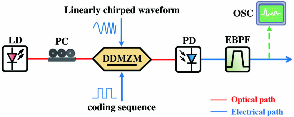
Fig. 1. Configuration of the proposed approach for the generation of switchable multi-format linearly chirped signals. LD, laser diode; PC, polarization controller; DDMZM, dual-drive Mach–Zehnder modulator; PD, photodetector; EBPF, electrical bandpass filter; OSC, oscilloscope.

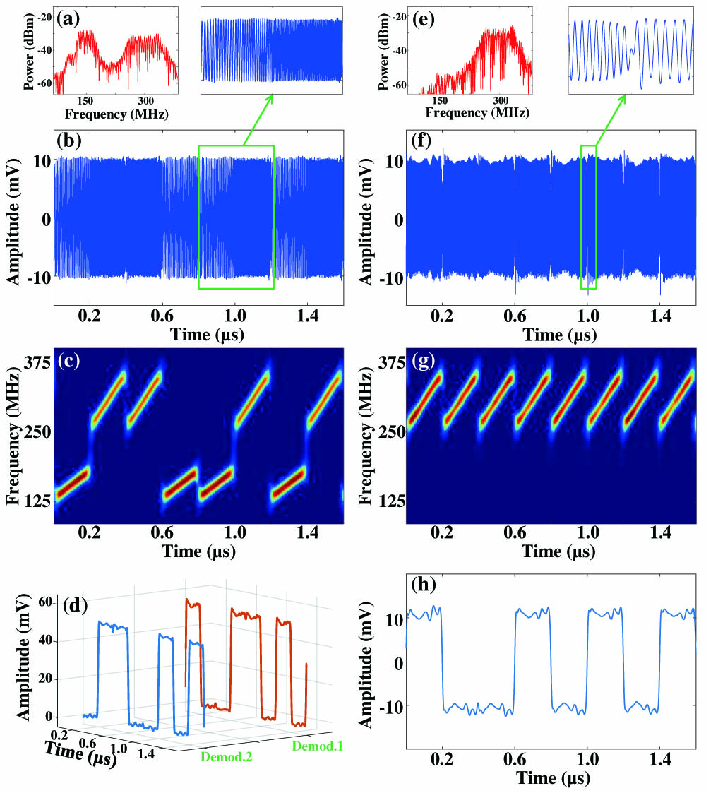
Fig. 2. Electrical spectra, time-domain waveform, frequency-time diagram, and recovered data of the generated linearly chirped signal with (a)–(d) FSK and (e)–(h) PSK formats. The coherent demodulation in (d) is, respectively, conducted by an LO with a frequency of 125–175 MHz (Demod.1) and 250–350 MHz (Demod.2).

Fig. 3. (a) Time-domain waveform, (b) electrical spectrum, (c), (d) frequency-time diagram, and (e), (f) recovered data of the generated dual-band linearly chirped signal with PSK format.

Fig. 4. (a) Time-domain waveform, (b) electrical spectrum, (c) frequency-time diagram, and (d) recovered data of the generated linearly chirped signal with the FSK/PSK format. The coherent demodulation is, respectively, conducted by an LO with a frequency of 125–175 MHz (Demod.1) and 250–350 MHz (Demod.2).

Fig. 5. (a) Electrical spectra without filtering. The green number n means the nth-order harmonic, and the red line depicts the amplitude response sketch of the EBPF. (b) The frequency-time diagram of the generated 5 Mbit/s 250–300/375–450 MHz FSK modulated linearly chirped signal.

Fig. 6. (a) Frequency-time diagram obtained by Hilbert transform in simulation. (b) The frequency-time diagram of the generated 100 Mbit/s 5–7/10–14 GHz FSK modulated linearly chirped signal with interference components.

Table 1. The Results of i2(t) Corresponding to Specific θ(t)