- Spectroscopy and Spectral Analysis
- Vol. 42, Issue 11, 3647 (2022)
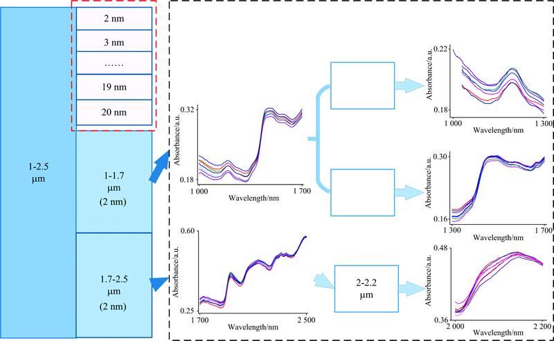
Fig. 1. Schematic diagram of analysis of different spectral bands and resolution
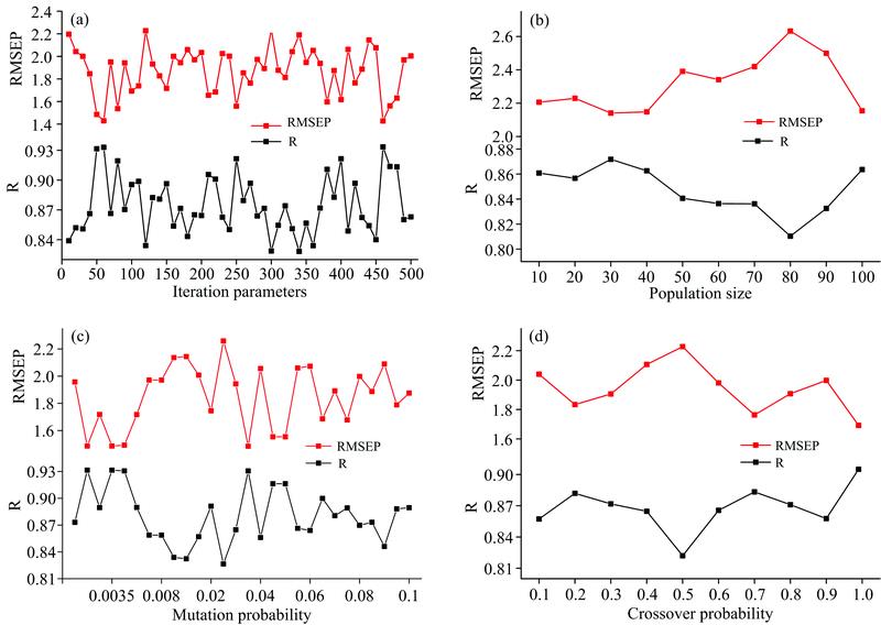
Fig. 2. Parameter selection of genetic algorithm
(a): Iteration parameters; (b): Population size; (c): Mutation probability; (d): Crossover probability
(a): Iteration parameters; (b): Population size; (c): Mutation probability; (d): Crossover probability
Fig. 3. Model prediction results of different spectral bands at the same resolution
Fig. 4. Model prediction results of different resolution at 1~2.5 μm spectral band
|
Table 1. Test results of different training functions
|
Table 2. Test results of different node transfer function


Set citation alerts for the article
Please enter your email address
© Copyright 2018-2021 | Chinese Laser Press. All Rights Reserved 沪ICP备15018463号-20