
Desheng Zeng, Li Zhong, Suping Liu, Xiaoyu Ma. Analysis of the time domain characteristics of tapered semiconductor lasers[J]. Journal of Semiconductors, 2020, 41(3): 032305
- Journal of Semiconductors
- Vol. 41, Issue 3, 032305 (2020)
Abstract
1. Introduction
Semiconductor lasers have compact structure, high photoelectric transformation efficiency and wide range of lasing wavelengths, so they have great application prospects in optical communication, laser processing, laser ranging, biomedical equipment and so on[
In this paper, we use traveling wave coupling theory to investigate the time domain characteristics of tapered semiconductor lasers with second order DBR gratings[
![]()
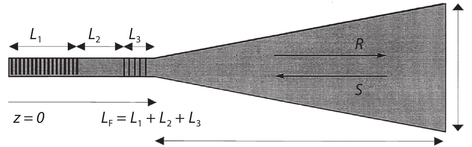
Figure 1.Schematic top view of the laser.
In the following section, the traveling wave theory and coupled mode equation are introduced and the finite difference method is used to solve the equation. In the third section, the simulation results are given, the variation of output optical power and charge carriers with time of tapered laser with DBR grating is analyzed, and the influence of different length front grating on longitudinal mode characteristics is compared. In the last section, the work of this paper is summarized.
2. Method
In semiconductor lasers with second order gratings, the coupling of the front and rear traveling waves must be considered. In this paper, R(t, z) stands for the forward wave, S(t, z) represents the backward wave, and the time domain coupling wave equation that they satisfy is as follows[
where vg represents the group velocity of the light wave, g represents the amplitude gain and phase change of the active region,
where
where A is the differential gain coefficient, N(z,t) is the carriers sheet density, N0 is the transparency sheet density. The last term of the coupled wave equation
where i represent R and S. The product of the upper formula and the lateral width W of the light field is the ratio of spontaneous emission to the forward wave or the backward wave.
As can be seen from this formula,
The time and spatial distribution of the carrier sheet N(t,z) is as follows:
where
Next, the finite difference method is used to solve the Eqs. (1a), (1b) and (6). Before that, the difference recurrence relation must be derived. Let
According to the slowly varying envelope approximation, the second order reciprocal of R to z can be ignored, and the following recurrence relation can be obtained:
where
where
According to the algorithm of differential matrix, the following results can be obtained:
where
Let matrix
Considering the effects of time and spontaneous emission, the final expression is obtained:
Boundary conditions:
where
The differential recurrence relationship of carriers is as follows:
where
3. Simulation results and analysis
In an ideal case, the reflectivity of the front cavity facet of the amplifier is zero, which would only display system dynamics originating in the master oscillator. The tapered amplify region amplifies the mode produced by the master oscillator region. In practice, the reflectivity of the front cavity surface is not zero, which will introduce additional models and aggravate the mode competition. For the noise term[
When the power reflectivity of the front-end face is 0.002 and the length of the front grating is 50 μm, as shown in Fig. 2, the carrier concentration of the device varies with time. In the first few nanoseconds, the carrier concentration rises sharply. The reason for this phenomenon is that the photons in the device have not yet been produced, and after the photons are excited, the carrier concentration decreases rapidly, and finally tends to be stable, and the generation of carriers and the transformation of photons reach a dynamic equilibrium. The following is the total number of photons in the device, which tends to be stable after the initial rapid change, slightly lagging behind the change of carrier concentration. Fig. 3 shows the spectrum after Fourier transform of the output light field power. As can be seen, there are multiple longitudinal mode patterns whose spacings are about 50 GHz when the device works stably, displaying serious mode competition between longitudinal modes.
![]()
Figure 2.(Color online) The top panel shows the change of total charge carriers and the bottom panel shows the change of total photons with the change of time with a 50
![]()
Figure 3.(Color online) The frequency of output light with a 50
Lengthening the front grating L3 can improve longitudinal mode characteristics. Increasing the front grating to 75 μm and the other conditions remain unchanged. It can be seen from the following figure that the number of longitudinal modes is obviously reduced, and the single longitudinal mode characteristics are more obvious with only three modes left, as shown in Fig. 4.
![]()
Figure 4.(Color online) The frequency of output light when front grating is 75
By extending the length of the grating L3 to 100 μm, we observe that the laser has high power and excellent longitudinal mode characteristics. In the simulation, mode competition occurs only in the first few nanoseconds. During this time, the master oscillator settles into a single longitudinal mode. As shown in Fig. 5, the above is the spectrum of the initial unstable state, and the below is the stable output spectrum.
![]()
Figure 5.(Color online) The top panel shows the transient frequency of output light during 0–5 ns and the bottom panel shows the stable state frequency of output light with a 100
Fig. 6 shows the variation of carriers and photons under the condition that the length of the front grating L3 is 100 μm. Fig. 7 shows the output power of the end facet, the output power above is the full time domain output power, and the bottom is the stable output power. As can be seen, under the stable condition, the output power tends to be stable. When the front grating is continued to increase to 200 μm, there is almost one longitudinal mode in the device (as shown in Fig. 8) but the power of the output light field is slightly lower than that of the front grating is 100 μm (as shown in Fig. 9).
![]()
Figure 6.(Color online) The top panel shows the change of total charge carriers and the bottom panel shows the total photons with a 100
![]()
Figure 7.(Color online) The top panel shows the change of output power with the change of time during all simulation time and the bottom panel shows the output power in stable state with a 100
![]()
Figure 8.(Color online) The stable state frequency of output light with a 200
![]()
Figure 9.(Color online) The top panel shows the change of output power with the change of time during all simulation time and the bottom panel shows the output power in stable state with a 200
From these frequency figures it can be found that along with the increase of the length of the front grating, there are fewer and fewer stable modes in the device. When the front grating is extended to 100 μm, almost one longitudinal mode exists in the compound-cavity, for which the front grating with suitable length can eliminate the mode degeneracy and ensure the stable operation of the single mode in the device.
4. Conclusion
We use coupled-wave equation to accurately analyze model the single longitudinal mode and the multiple longitudinal mode in a compound cavity. The integration algorithms in Eq. (12) can help us to take larger time steps while maintaining computational efficiency and accuracy. To get nearly ideal single longitudinal mode and high-power output, we optimize the length of front gratings. When the front grating is extended to no less than 100 μm, mode competition occurs over only the first few nanoseconds, at which time the master oscillator settles into a single longitudinal mode. Meanwhile, considering that the structure scale of the laser must be controlled in a certain range and maintain its high photoelectric transformation efficiency, the grating length cannot be too long to avoid affecting its practicability. Therefore, the ideal light output can be obtained by increasing the length of front grating to about 100 μm, when MO and PA area are driven separately using different electrodes[
The calculated results in this paper have significance for the actual fabrication of tapered lasers with DBR gratings. The model that we have developed in this article can be used to analyze 3D simulations when lateral and transverse optical fields are considered[
References
[1] S M Sun, J Fan, L Xu et al. Research progress of conical semiconductor lasers. Chin Opt, 12, 48(2019).
[2] X Y Zhou, S Y Zhao, X L Ma et al. Low vertical divergence angle high brightness photonic crystal semiconductor laser. Chin J Lasers, 44, 0201010(2017).
[3] Y Q Liu, Y H Cao, J Li et al. 5 kW fiber coupled semiconductor laser for laser processing. Opt Prec Eng, 23, 1279(2015).
[4] K Paschke, B Sumpf, F Dittmar et al. Nearly diffraction limited 980-nm tapered diode lasers with an output power of 7.7 W. IEEE J Sel Top Quantum Electron, 11, 1223(2005).
[5] P Jia, X L Liu, Y Y Chen et al. Study of dual wavelength distributed Bragg reflection semiconductor laser with high order Bragg gratings. Chin J Lasers, 37(2015).
[6] A T Aho, J Viheriälä, Korpijärvi V M M et al. High-power 1180-nm GaInNAs DBR laser diodes. IEEE Photonics Technol Lett, 29, 2023(2017).
[7] J Fan, C Y Gong, J J Yang et al. Research progress of distributed prague reflector semiconductor lasers. Progr Laser Optoelectron, 56, 34(2019).
[8] A Müller, J Fricke, F Bugge et al. DBR tapered diode laser with 12.7 W output power and nearly diffraction-limited, narrowband emission at 1030 nm. Appl Phys B, 122, 87(2016).
[9] H Kogelnik, C V Shank. Coupled-wave theory of distributed feedback lasers. J Appl Phys, 43, 2327(1972).
[10] G C Dente, M L Tilton. Modeling multiple-longitudinal-mode dynamics in semiconductor lasers. IEEE J Quantum Electron, 34, 325(1998).
[11] K H Hasler, H Wenzel, A Klehr et al. Simulation of the generation of high-power pulses in the GHz range with three-section DBR lasers. IEE Proceedings-Optoelectronics, 149, 152(2002).
[12] M Radziunas. Modeling and simulations of broad-area edge-emitting semiconductor devices. Intl J High Perform Comput Appl, 32, 512(2018).
[13] K Vahala, A Yariv. Semiclassical theory of noise in semiconductor lasers-Part I. IEEE J Quantum Electron, 19, 1096(1983).
[14] K Vahala, A A Yariv. Semiclassical theory of noise in semiconductor lasers-Part II. IEEE J Quantum Electron, 19, 1102(1983).
[15] L M Zhang, S F Yu, M C Nowell et al. Dynamic analysis of radiation and side-mode suppression in a second-order DFB laser using time-domain large-signal traveling wave model. IEEE J Quantum Electron, 30, 1389(1994).
[16]
[17] A M De Melo, K Petermann. On the amplified spontaneous emission noise modeling of semiconductor optical amplifiers. Opt Commun, 281, 4598(2008).
[18] D Marcuse. Computer simulation of laser photon fluctuations: Theory of single-cavity laser. IEEE J Quantum Electron, 20, 1139(1984).
[19] L Borruel, H Odriozola, J M G Tijero et al. Design strategies to increase the brightness of gain guided tapered lasers. Opt Quantum Electron, 40, 175(2008).
[20] M Spreemann, M Lichtner, M Radziunas et al. Measurement and simulation of distributed-feedback tapered master-oscillator power amplifiers. IEEE J Quantum Electron, 45, 609(2009).
[21] C Qiao, R G Su, X Li et al. Design and technology of 980 nm high power DBR semiconductor laser. Chin Laser, 46, 0701002(2019).
[22] W X Wang, Y X Lu. Analysis of sampling grating characteristics of distributed feedback semiconductor lasers. Laser J, 39, 57(2018).

Set citation alerts for the article
Please enter your email address
© Copyright 2018-2021 | Chinese Laser Press. All Rights Reserved 沪ICP备15018463号-20