Nonlinear gallium phosphide nanoscale photonics [Invited]

Aude Martin; Sylvain Combrié; Alfredo de Rossi; Grégoire Beaudoin; Isabelle Sagnes; Fabrice Raineri

doi:10.1364/PRJ.6.000B43

Journals >Photonics Research >Volume 6 >Issue 5 >Page B43 > Article

Photonics Research
Vol. 6, Issue 5, B43 (2018)

Nonlinear gallium phosphide nanoscale photonics [Invited]

Aude Martin^1、2, Sylvain Combrié², Alfredo de Rossi^2、*, Grégoire Beaudoin¹, Isabelle Sagnes¹, and Fabrice Raineri^1、3

Author Affiliations

¹Centre de Nanosciences et de Nanotechnologies, CNRS, Université Paris-Sud, Université Paris-Saclay, C2N Marcoussis, 91460 Marcoussis, France

²Thales Research and Technology France, 1 avenue Augustin Fresnel, 91120 Palaiseau, France

³Université Paris Diderot, Sorbone Paris Cité, 75013 Paris, France

show less

DOI: 10.1364/PRJ.6.000B43 Cite this Article Set citation alerts

Aude Martin, Sylvain Combrié, Alfredo de Rossi, Grégoire Beaudoin, Isabelle Sagnes, Fabrice Raineri. Nonlinear gallium phosphide nanoscale photonics [Invited][J]. Photonics Research, 2018, 6(5): B43 Copy Citation Text

EndNote(RIS)

BibTex

Plain Text

show less

(a) SEM image of a PhC waveguide made of a GaP slab and close-up before the removal of the etching mask (red rectangle). The waveguide design (blue rectangle) indicates the relevant parameters, the radius of the holes, r; the period of the triangular lattice, a; the width of the defect line, W; and the transverse shift of the first row of holes, s. (b) Calculated (dashed) and measured (solid thick) average group index. The thin blue solid line is the calculated group index in the slow section. The cyan circle corresponds to the FWM experiment (ng=19). (c) Corresponding second-order dispersion (same codes). (d) Transmission spectrum, including fiber-to-waveguide coupling (dashed line represents insertion losses). The red lines are a guide for the eyes.

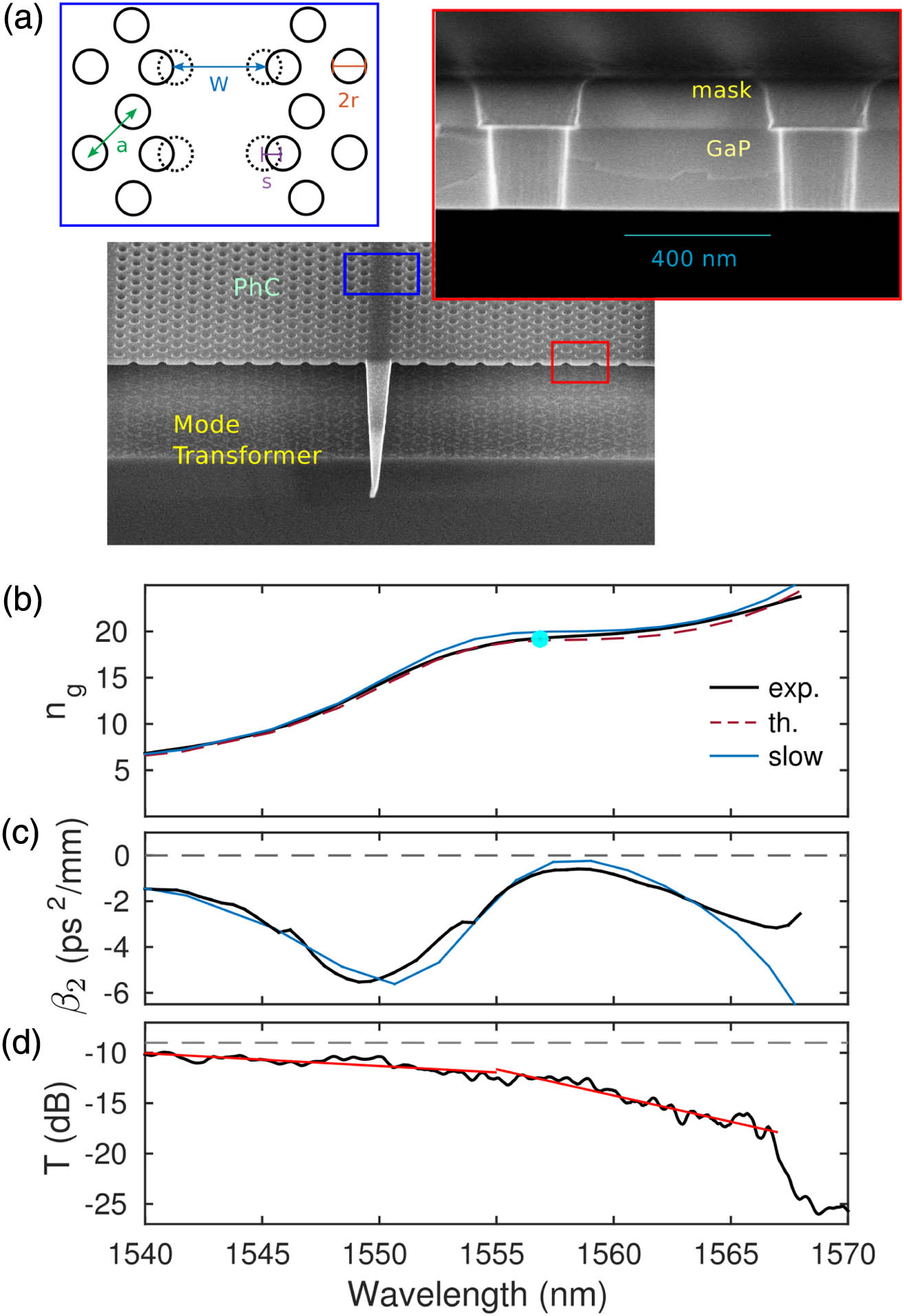
Fig. 1. (a) SEM image of a PhC waveguide made of a GaP slab and close-up before the removal of the etching mask (red rectangle). The waveguide design (blue rectangle) indicates the relevant parameters, the radius of the holes, r; the period of the triangular lattice, a; the width of the defect line, W; and the transverse shift of the first row of holes, s. (b) Calculated (dashed) and measured (solid thick) average group index. The thin blue solid line is the calculated group index in the slow section. The cyan circle corresponds to the FWM experiment (ng=19). (c) Corresponding second-order dispersion (same codes). (d) Transmission spectrum, including fiber-to-waveguide coupling (dashed line represents insertion losses). The red lines are a guide for the eyes.

Download full size | View in the Article

Picosecond pulse propagation and soliton dynamics. (a) Autocorrelation traces, experimental (grey circles) and calculated (red line). (b) Corresponding experimental output (grey circles) and input (cyan line) spectra. The calculated output spectrum (solid red line) is also represented with the calculated input one (dashed black line). (c) Calculated evolution of the pulse at some specified positions inside the waveguide. (d) Evolution of peak power P, pulse energy W, and duration Δt.

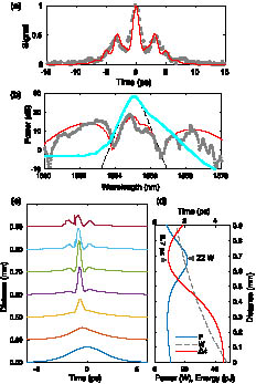
Fig. 2. Picosecond pulse propagation and soliton dynamics. (a) Autocorrelation traces, experimental (grey circles) and calculated (red line). (b) Corresponding experimental output (grey circles) and input (cyan line) spectra. The calculated output spectrum (solid red line) is also represented with the calculated input one (dashed black line). (c) Calculated evolution of the pulse at some specified positions inside the waveguide. (d) Evolution of peak power P, pulse energy W, and duration Δt.

Download full size | View in the Article

Fig. 3. (a) Measurement of the nonlinear absorption for ng=11 through the plot of the inverse transmission versus the peak power T0T=1+2I(γ)PLeff in the waveguide. (b) Nonlinear phase shift ϕNL. (c) Calculated inverse linear and nonlinear cross sections Aeff and 1/Aχ(3) as a function of the group index (see Appendix A). (d) Nonlinear parameter γ versus group index. Estimate from the spectral broadening (magenta squares), values used in the model (green circles), and calculated (solid line) using n2=3.5×10−18 W−1·m−2. The dashed red line represents the ng2 dependence as a guide for the eyes.

Download full size | View in the Article

Fig. 4. Four-wave mixing experiment with ps pulses at 2 GHz rate. (a) Output spectra corresponding to two different coupled peak power levels and spectrum of the pump at input. (b) Measured conversion efficiency as a function of the pump-probe detuning as the pump power is increased. The colored solid lines stand for the theory. The peak conversion efficiency η is plotted versus the pump power in the inset and compared with the model (solid lines), which also provides the parametric gain G. Filled circles correspond to the plots according to the color code.

Download full size | View in the Article

Fig. 5. Cascaded four-wave mixing experiment with ns pulses. (a) Output spectra and (b) raw conversion efficiency (ηL) as a function of the peak power. The dashed line corresponds to η∝P2. Detail of (c) the output and (d) the input at maximum peak power: experimental (red) and calculated (black) spectra.

Download full size | View in the Article

Geom. Mat. Exp. Refs.		PhC GaInP Membr. FWM [20]	Sol [21]	PhC GaInP on ${SiO}_{2}$ FWM [22]	PhC GaP Membr. [This Work]		PhC Si on ${SiO}_{2}$ FWM [23]	FWM (Sol) [24]	Wire $α - Si$ on ${SiO}_{2}$ Sol [3]	FWM [25]	Wire AlGaAs on ${SiO}_{2}$ FWM [26]
Geom. Mat. Exp. Refs.		PhC GaInP Membr. FWM [20]	Sol [21]	PhC GaInP on ${SiO}_{2}$ FWM [22]	FWM	Sol	PhC Si on ${SiO}_{2}$ FWM [23]	FWM (Sol) [24]	Wire $α - Si$ on ${SiO}_{2}$ Sol [3]	FWM [25]	Wire AlGaAs on ${SiO}_{2}$ FWM [26]
$Δ t$	ps	30	2	CW	4	15	CW	CW (1)	1.8	3.8	CW
$ζ$	%	0.5	0.007	100	3	0.015	100	100 (0.002)		0.004	100
$P$	W	0.8	10		4.5	20†		(30)		5.3	1.5
$\bar{P}$	mW	4	0.8	100	135	1.7	90	20 (0.6)	3	0.2	1.5
$I$	$GW / {cm}^{2}$		$\approx 10$		12	50†		$\approx 30$	4	$\approx 5$	$\approx 0.75$
$\bar{I}$	$MW / {cm}^{2}$	$\approx 10$		$\approx 600$	400		$\approx 600$	20		$≪ 1$	$\approx 750$
$A_{eff}$	${μm}^{2}$			$\approx 0.03$	0.04	0.04	$\approx 0.03$	$\approx 0.1$	$< 0.1$	$< 0.1$	$\approx 0.2$
$A_{χ^{(3)}}$	${μm}^{2}$	0.004	0.02	0.006	0.01	0.015	0.006	0.21	0.07	0.07	0.14
$n_{g}$		15	9	30	20	15	30	3.5	3.5	3.5	3
$n_{2}$	$10^{- 17} W^{- 1} \cdot m^{- 2}$	0.7		0.7	0.35		$\approx 0.6$	1.7	2.1	1.3	2.5
$α$	$dB / cm$	$0.1 n_{g}^{2}$		$< 0.1 n_{g}^{2}$	$0.16 n_{g}^{2}$		$< 0.1 n_{g}^{2}$	4	4.5	4.8	1.5
$η$	dB	5	n.a.	−18	0.8	n.a.	−24	−21	n.a.	$+ 26$	$> 0$
$γ$	$W^{- 1} \cdot m^{- 1}$	6000	1000	4500	1600	1000	4000	330	1200	770	650
$γ / α$	$W^{- 1}$	6	1.5	2.5	1.5	1	2.5	4	12	7	$> 20$
F		$≫ 1$		$≫ 1$	$1.5 \pm 0.5$		0.4 (TE)	5 (TM)	5 (TE)	2 (TE)	$≫ 1$