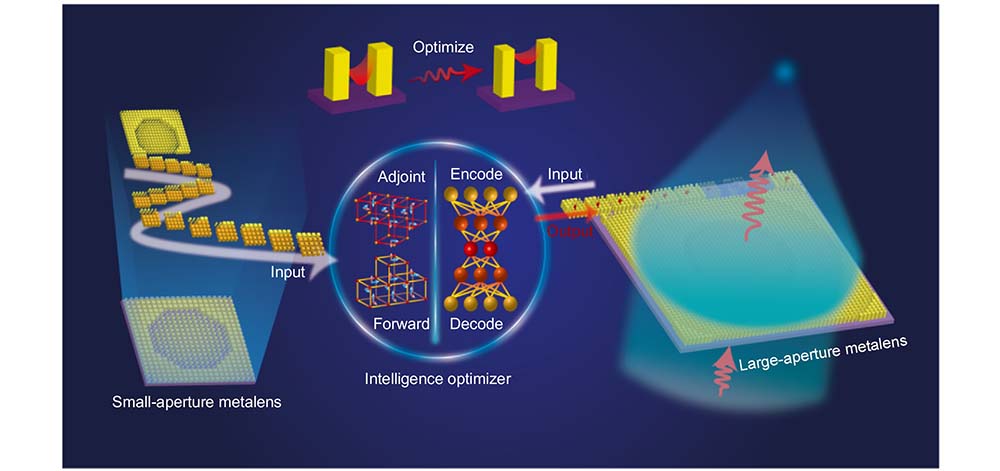
Fig. 1. Working principle of the “intelligent optimizer”. The “intelligent optimizer” incorporates both Adj and DL methods. Data-sets of the DL network are obtained from the small-aperture metalens optimized by the Adj method. Super meta-atoms of large-aperture metalens are fed into the network one by one. Output meta-atoms are spliced together to create a new metalens with improved focusing efficiency.

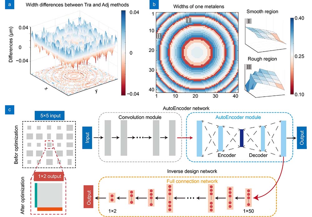
Fig. 2. Design method for the large-aperture metalens. (a) The differences in widths distribution for the meta-atoms before and after optimization. (b) The widths distribution of metalens, with the smooth region and rough region corresponding to translucent boxes I and II, respectively. (c) The optimized network framework consists of an A-network that expands the information space of sampled data, and the weak coupling strength structures are filtered by the I-network.

Fig. 3. Simulation results of Adj and DL methods. (a) Electric field distributions in the xy and xz planes designed by DL method for x- and y-polarized light, and the Adj method for x-polarized, respectively. (b) Electric intensity profiles of the focal spot designed by theory, Adj, and DL methods, respectively. (c) Width distributions of metalenses on y=0 plane (x>0) designed by the traditional (Tra), Adj, and the proposed methods, respectively. (d) Width differences between the initial metalens and the optimized metalenses designed by the Adj method and our methods.

Fig. 4. Experimental results of optimized metalenses. (a) The left image shows an overview of the device, with each diameter corresponding to four exposure doses. The inset is the optical microscope image. Scale bar: 100 µm. The right image is the scanning electron microscope image. Scale bar: 2 µm. (b) The first row shows the focal plane intensity distributions of the three metalenses (100.5 μm, 500 μm, and 1 mm, from left to right, respectively). The second row shows the normalized focal intensity along the x-axis at the focal plane of the three metalenses. (c) Focal intensity distributions in the xz plane at the three metalenses. (d) Relative focusing efficiencies and Strehl ratios of three metalenses. (e) Imaging results of elements #5 and #6 from group #7 of the USAF resolution target at 1 mm diameter optimized metalens (left) and 1 mm diameter ideal metalens (right). Scale bar: 5 µm.

Table 1. Examples to show the representative parameters and performance of various methods.