
Hongxia Yang, Hao Guo, Yan Gao, Jubai An. SAR Flow Ice Separation Algorithm Combined with Saliency Detection[J]. Laser & Optoelectronics Progress, 2020, 57(20): 201010
- Laser & Optoelectronics Progress
- Vol. 57, Issue 20, 201010 (2020)
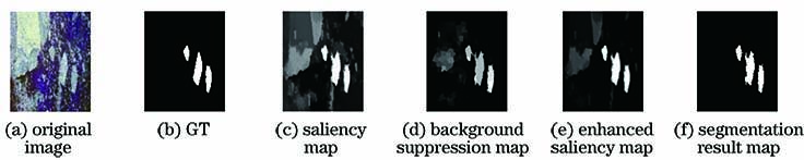
Fig. 1. Experimental intermediate diagram
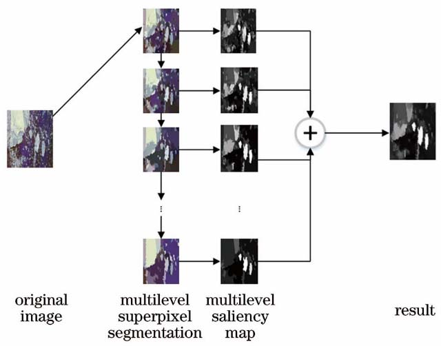
Fig. 2. Calculation process of saliency maps
Fig. 3. Three-dimensional color histograms of different regions. (a) Sea ice; (b) sea water; (c) crushed ice
Fig. 4. Saliency maps obtained by different algorithms. (a) Original image; (b) GT; (c) DRFI; (d) RBD; (e) MR; (f) GS; (g) BSCA; (h) MAP; (i) SRD; (j) proposed algorithm
Fig. 5. Comparison of P-R curves of different algorithms
Fig. 6. Comparison of MAE values of different algorithms
Fig. 7. MAE in different datasets
Fig. 8. F_measure in different datasets
Fig. 9. Comparison of segmentation methods. (a) Original image; (b) GT; (c) proposed algorithm; (d) MACWE; (e) MRF; (f) MRF_BCD
Fig. 10. MIoU of each segmentation method
|
Table 1. Information table of seascape images
|
Table 2. Running time of different algorithms
|
Table 3. Comparison of F_measure values of different algorithms

Set citation alerts for the article
Please enter your email address
© Copyright 2018-2021 | Chinese Laser Press. All Rights Reserved 沪ICP备15018463号-20