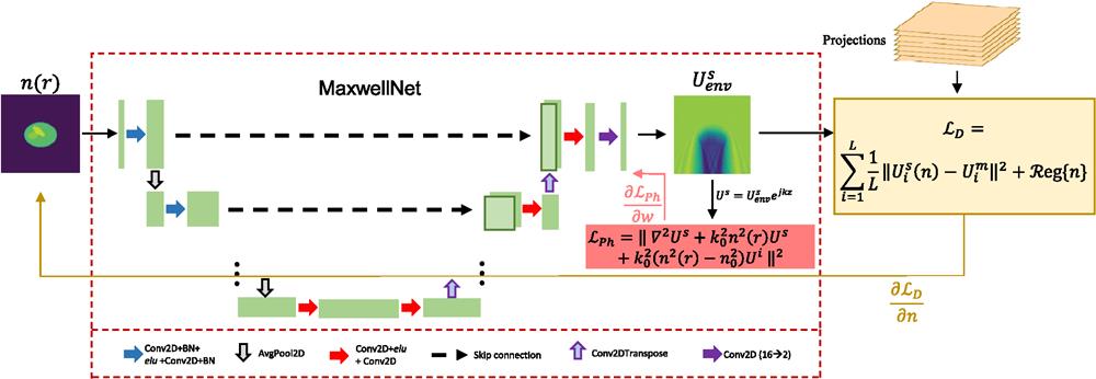
Fig. 1. Schematic description of MaxwellNet, with U-Net architecture, and its application for tomographic reconstruction. The input is a refractive index distribution and the output is the envelope of the scattered field. The output is modulated by the fast-oscillating term ejk0n0z to compute the physics-informed loss for tuning the weights. For tomographic reconstruction, we minimize a data-driven loss based on the difference between measured and calculated projections using MaxwellNet. A regularization term can be added to improve the reconstruction.

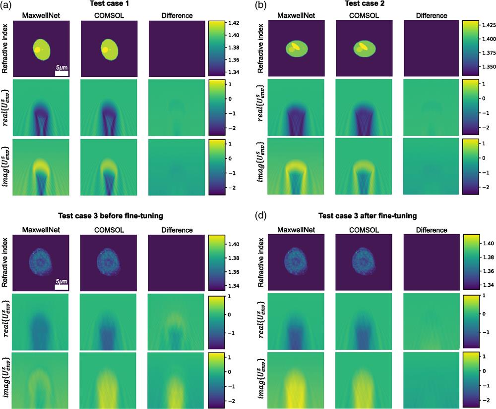
Fig. 2. Results of MaxwellNet and its comparison with COMSOL. (a) and (b) Two test cases from the digital phantom dataset and the prediction of the real and imaginary parts of the envelope of the scattered fields using MaxwellNet, COMSOL, and their difference. (c) Scattered field predictions from the network trained in (a) and (b) for the case of an experimentally measured RI of HCT-116 cancer cells and comparison with COMSOL. The difference between the two is no longer negligible. (d) Comparison between MaxwellNet and COMSOL after fine-tuning the former for a set of HCT-116 cells. MaxwellNet predictions reproduces much more accurate results after fine-tuning.

Fig. 3. Results of 3D MaxwellNet and its comparison with COMSOL. The RI distribution is shown in (a). The real part of the envelope of the scattered field calculated by 3D MaxwellNet is shown in (b), calculated by COMSOL in (c), and their difference in (d). The imaginary part of the envelope of the scattered field calculated by 3D MaxwellNet, COMSOL, and their difference are presented in (e)–(g), respectively.

Fig. 4. Tomographic reconstruction of RI using MaxwellNet. (a) The RI reconstruction was achieved by Rytov, MaxwellNet, and the ground truth. (b) 1D RI profile at z=0 (plane of best focus), for Rytov (green), MaxwellNet (blue), and the ground truth (orange).

Fig. 5. Tomographic RI reconstruction of 3D sample using MaxwellNet. The RI reconstruction is achieved by Rytov, MaxwellNet, learning tomography, and the ground truth in different rows at the YX, YZ, and XZ planes in the center of the sample. A z-stack demonstration of the reconstruction is shown in Video 1 (Video 1, MP4, 1.4 MB [URL: https://doi.org/10.1117/1.AP.4.6.066001.s1]).

Fig. 6. Tomographic RI reconstruction of a polystyrene microsphere immersed in water. The projections are measured with off-axis holography for different angles. The RI reconstructions achieved by Rytov, MaxwellNet, and learning tomography are presented at the YX, YZ, and XZ planes in the center of the sample, respectively.

Fig. 7. Training and fine-tuning of MaxwellNet. (a) Training (blue) and validation (orange) loss of MaxwellNet for the digital cell phantoms dataset. (b) Fine-tuning of the pretrained MaxwellNet for a dataset of HCT-116 cells for 1000 epochs. (c) Examples of the HCT-116 dataset.

Fig. 8. Experimental setup for multiple illumination angle off-axis holography. HW: half-wave plate; P: polarizer; BS: beam splitter; L: lens; Obj: microscope objective; and M: mirror.

Table 1. Computation time comparison.