
Yanqiong Shi, Qiuxia Ying, Rongsheng Lu. Performance Analysis of Three-Dimensional Measurement Algorithm with Focus Variation Microscopic Imaging[J]. Laser & Optoelectronics Progress, 2019, 56(7): 071202
- Laser & Optoelectronics Progress
- Vol. 56, Issue 7, 071202 (2019)
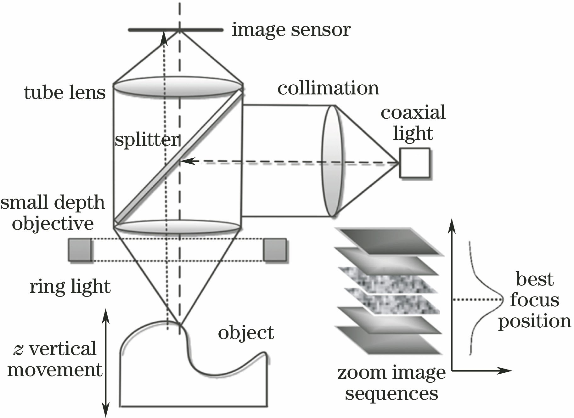
Fig. 1. Schematic of focus variation
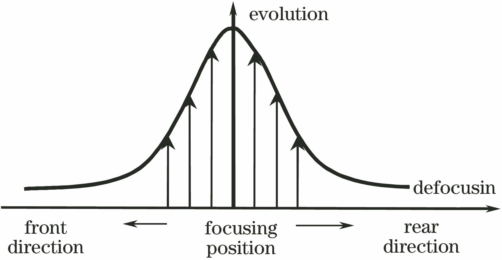
Fig. 2. Ideal focusing curve
Fig. 3. An experimental image obtained using focus variation microscopy and three testing points
Fig. 4. Focus curves obtained from single point information and neighborhood information with different operators. (a) Brenner operator; (b) Roberts operator; (c) Laplace operator; (d) Tenengrad operator; (e) SMD operator; (f) gradient square; (g) Sobel operator in eight directions
Fig. 5. Focus scatter plots with different sizes of neighborhood. (a) 5; (b) 9; (c)13; (d) 17
Fig. 6. Focusing evaluation results of points with different brightness. (a) (380,280); (b) (700,390); (c) (608,218)
Fig. 7. Focusing evaluation results of three brighter points. (a) (765,115); (b) (363,1095); (c) (829,68)
Fig. 8. Schematic of wavelet fusion method
Fig. 9. Comparison of image fusion results. (a) Image fusion based on spatial regional characteristics; (b) image fusion with frequency domain wavelet; (c) color image fusion with frequency domain wavelet
Fig. 10. Experimental system
Fig. 11. Image sequence diagrams of coin surface. (a) 1st image; (b) 2nd image; (c) 30th image; (d) 31st image; (e) 80th image; (f) 81st image
Fig. 12. 3D measurement results of coin surface relief. (a) 3D point cloud; (b) 3D color reconstruction image
Fig. 13. A gauge step measurement result. (a) One of images in image sequence; (b) 3D point cloud data; (c) point cloud distribution of a section
| ||||||||||||||||||||||||||
Table 1. Time consumed per image during focus evaluation by using single point and neighborhood information
|
Table 2. Time consumed per image during focus evaluation with different sizes of neighborhood
|
Table 3. Comparison of results obtained by different extremum searching methods

Set citation alerts for the article
Please enter your email address
© Copyright 2018-2021 | Chinese Laser Press. All Rights Reserved 沪ICP备15018463号-20