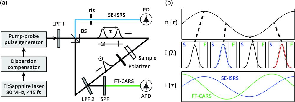
Fig. 1. Schematic and principle of DIVS. (a) Optical setup for DIVS. Following dispersion compensation and a pump–probe generator, cross-polarized pump and probe pulses with variable delay ($\tau$) are longpass filtered (LPF 1) and split at a BS into CW and CCW paths within an SI. In the CW path, the probe phase is modulated with $\tau$ dependence at the sample. A polarizer eliminates the pump pulse. At LPF 2 within the SI, a fraction of the probe is reflected to be detected as FT-CARS after an SPF. The rest of the probe interferes at the upper side of the BS with the LO generated in the CCW direction, generating the SE-ISRS signal. An iris is used to select a high-SNR region of the signal. (b) Principles of DIVS signals. At the sample, the pump pulse causes the refractive index to oscillate in time (upper panel). The $\tau$-dependent phase modulation of a following probe results in either a spectral shift (detected in FT-CARS via filtering) or a phase delay shift (detected in SE-ISRS via interference), according to the slope of the refractive index (middle panel). Vertical lines in each spectrum indicate the optical filter cutoff separating the SE-ISRS (S) and FT-CARS (F) detection regions. The FT-CARS signal is proportional to the temporal derivative of the refractive index, while the SE-ISRS signal is proportional to the refractive index itself (lower panel). This key difference provides the complementary THz and fingerprint sensitivities of SE-ISRS and FT-CARS, respectively.

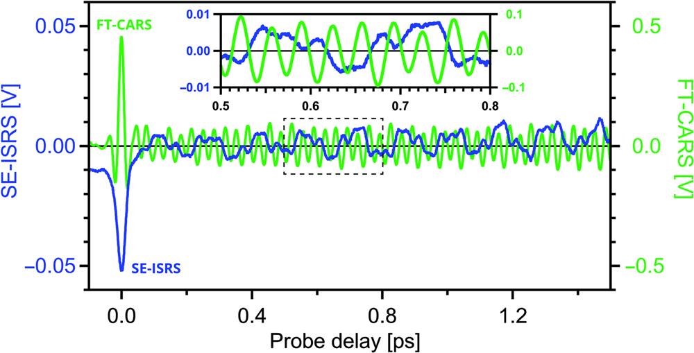
Fig. 2. Time-domain DIVS signals. SE-ISRS (blue, left axis) and FT-CARS (green, right axis) time-domain signals were simultaneously acquired in less than $42\mu \mathrm{s}$. The zoomed-in inset corresponds temporally to the region outlined in the dashed rectangle. In the SE-ISRS signal, lower-frequency Raman modes are dominant, while higher-frequency modes are comparatively stronger in the FT-CARS signal.

Fig. 3. Waterfall plots of (a) SE-ISRS and (b) FT-CARS spectra obtained at $\mathrm{24,000}\text{spectra}/\mathrm{s}$. The sample is a 1:1 (volume ratio) mixture of bromoform and benzene. Insets show a plot of 1500 averaged spectra. Individual spectra in the waterfall plots are normalized to the average power of the noise region of 2000 to $2400{\mathrm{cm}}^{-1}$ in the corresponding 1500-spectra average plot. The lowest-frequency mode of bromoform at $154{\mathrm{cm}}^{-1}$ is detected in individual SE-ISRS spectra but not detected in individual FT-CARS spectra. The ${1178\text{-}\mathrm{cm}}^{-1}$ mode of benzene is detected in individual FT-CARS spectra but not detected in individual SE-ISRS spectra. The plots highlight the complementary nature of both signals.

Fig. 4. Comparison of SE-ISRS and FT-CARS spectral sensitivities in DIVS. Plotted are the ratios of the average SNRs of SE-ISRS and FT-CARS signal powers of the Raman-active modes of bromoform, benzene, toluene, and tetrabromoethane as measured by DIVS (left axis). A dashed line shows equivalence between SE-ISRS and FT-CARS SNRs (left axis). The solid line indicates the theoretical ratio of SE-ISRS and FT-CARS powers in DIVS (right axis).

Fig. 5. Waterfall plots of (a) SE-ISRS and (b) FT-CARS spectra of bromoform. Spectra were obtained at $\mathrm{24,000}\text{spectra}/\mathrm{s}$. Insets show a plot of 1500 averaged spectra. Individual spectra in the waterfall plots are normalized to the average power of the noise region of 2000 to $2400{\mathrm{cm}}^{-1}$ in the corresponding 1500-spectra average plot.

Fig. 6. Waterfall plots of (a) SE-ISRS and (b) FT-CARS spectra of benzene. Spectra were obtained at $\mathrm{24,000}\text{spectra}/\mathrm{s}$. Insets show a plot of 1500 averaged spectra. Individual spectra in the waterfall plots are normalized to the average power of the noise region of 2000 to $2400{\mathrm{cm}}^{-1}$ in the corresponding 1500-spectra average plot.

Fig. 7. Waterfall plots of (a) SE-ISRS and (b) FT-CARS spectra of toluene. Spectra were obtained at 24,000 spectra/s. Insets show a plot of 1500 averaged spectra. Individual spectra in the waterfall plots are normalized to the average power of the noise region of 2000 to $2400{\mathrm{cm}}^{-1}$ in the corresponding 1500-spectra average plot.

Fig. 8. Waterfall plots of (a) SE-ISRS and (b) FT-CARS spectra of tetrabromoethane. Spectra were obtained at $\mathrm{24,000}\text{spectra}/\mathrm{s}$. Insets show a plot of 1500 averaged spectra. Individual spectra in the waterfall plots are normalized to the average power of the noise region of 2000 to $2400{\mathrm{cm}}^{-1}$ in the corresponding 1500-spectra average plot.

Fig. 9. Concentration-dependent plot of the SNR of SE-ISRS and FT-CARS signals. The FT-CARS SNR (green) is represented as the SNR of the $992\text{-}{\mathrm{cm}}^{-1}$ mode of benzene, while the SE-ISRS SNR (blue) is represented as the SNR of the $222\text{-}{\mathrm{cm}}^{-1}$ mode of bromoform. SNR values were calculated as the average of 15,000 spectra obtained at $\mathrm{24,000}\text{spectra}/\mathrm{s}$.

Fig. 10. Simulated frequency-dependent plot of the normalized power of SE-ISRS and FT-CARS signals in DIVS. The SE-ISRS power (blue) dominates in the low-frequency Raman spectral region, whereas the FT-CARS power (green) is higher in the fingerprint region.

Table 1. Mean ratios of the SNRs of SE-ISRS (SE) and FT-CARS (FT) and their standard deviations (n=10).

Table 2. Average SNRs and standard deviations (n=10) from individual spectra of bromoform and benzene.

Table 3. Average SNRs and standard deviations (n=10) from individual spectra of toluene.

Table 4. Average SNRs and standard deviations (n=10) from individual spectra of tetrabromoethane.