Raman spectroscopy enables the acquisition of chemically specific vibrational information from target samples without the use of chemical labels. These features have established Raman spectroscopy as a ubiquitous tool with valuable applications across a diverse range of academic and industrial fields, such as material science,1^–3 biology,4^–6 pharmaceuticals,7^–9 and medicine.10^,11 Raman spectra are generally partitioned into three regions: (1) the “high-frequency” region (2400 to 4000cm−1) containing C—H and O—H stretching vibrations; (2) the “fingerprint” region (200 to 1800cm−1) containing signature intramolecular bond vibrations; and (3) the “low-frequency” or “terahertz” (THz) region (<200cm−1, <6THz) containing intermolecular vibrations. In particular, the fingerprint and THz regions are highly valuable when measured in concert via broadband detection (>1000cm−1); together the two regions provide both chemically specific information about the molecular content of a sample, as well as insights into the behavior of groups of molecules. This can be especially valuable in fields such as pharmacology or polymer research, where the purity or localization of targets may be assessed by fingerprint spectra, while the crystalline polymorphism or the polymer stress, extent, or nature of polymerization can be probed by low-frequency spectra.12^–17

Although there exist a multitude of techniques for capturing broadband Raman spectra across the THz–fingerprint region, they tend to be too slow for certain applications. For example, spontaneous Raman spectroscopy, a well-developed and commonly used Raman technique, can provide broadband vibrational spectra including both low-frequency and fingerprint regions but at typical spectral acquisition rates of <10spectra/s. Similarly, alternative vibrational spectroscopy techniques, such as impulsive stimulated Raman scattering (ISRS) spectroscopy,18^–21 optical Kerr effect spectroscopy,22^–24 Raman-induced Kerr effect spectroscopy25^–28, Raman-induced Kerr lensing with impulsive excitation,29 and radio frequency Doppler Raman spectroscopy,30 can provide broadband spectra across the THz–fingerprint region. However, such techniques typically offer spectral acquisition rates of <10spectra/s due to reliance on slow methods for increasing the Raman spectral signal-to-noise ratio (SNR), such as longer integration times or slow probe delay scanning. Despite the rich information provided by these and other broadband THz–fingerprint Raman techniques, they are unsuitable for certain applications that demand higher spectral acquisition rates, such as video-rate vibrational imaging or detecting rapid transient phenomena.

On the other hand, there are methods for capturing either THz or fingerprint spectra independently but at higher speeds. For example, Raanan et al. demonstrated a method for sub-second hyperspectral Raman microscopy, which was enabled by impulsive low-frequency Raman spectroscopy at 40,000spectra/s.31 With this technique, high-speed pump–probe delay scanning of 160-fs pulses was performed with an acousto-optic programmable dispersive filter (AOPDF), such that high sensitivity in the low-frequency region was achieved by detecting time-domain vibrational signals which are sensitive to both the sample refractive index (via Raman-induced Kerr lensing) and its time derivative (via Raman-induced spectral shifting). However, the method’s reliance on an AOPDF delay line, which is not compatible with short pulse widths in the sub-30-fs regime,32 prevents broadband detection including the fingerprint region. In another report, Domingue et al. demonstrated a technique for low-frequency Raman spectroscopy at a spectral acquisition rate up to 700 Hz, which uses a spinning window for rapid ISRS pump–probe delay scanning and optical bandpass filtering with balanced detection to measure the time-domain Raman signals.33 However, the technique relies on high-gain amplified balanced detection, the low bandwidth of which limits concurrent measurement of the fingerprint region. Likewise, techniques, such as Fourier-transform coherent anti-Stokes Raman scattering (FT-CARS) spectroscopy,34^–37 dual-comb CARS,38^–40 and quasi-dual-comb CARS,41 can provide broadband fingerprint spectra with ultrafast spectral acquisition rates ranging from 10,000 to 100,000spectra/s. These techniques detect molecular vibrations via the frequency shift of the probe but are differentiated from ISRS spectroscopy, especially by their use of optical long- and short-pass filtering to eliminate the large probe background noise in ISRS and isolate the Raman signal. While the resultant high SNR of this approach enables ultrafast probe delay scanning and spectral acquisition rates above 10,000spectra/s, these methods cannot access the low-frequency Raman region due to the attenuation of low-frequency modes by the optical short-pass filtering as well as detection schemes based on frequency-shifted probe signals, the strength of which in the low-frequency region by nature decreases as the detected Raman frequency decreases.

To address the current limitations of high-speed broadband Raman spectroscopy, in this paper, we present dual-detection impulsive vibrational spectroscopy (DIVS), a straightforward single-laser technique for broadband THz–fingerprint measurements at a spectral acquisition rate of 24,000spectra/s. This is achieved by a design enabling ultrafast measurement of both FT-CARS and Sagnac-enhanced ISRS (SE-ISRS,42 or “phase-sensitive” ISRS43), simultaneously. In DIVS, FT-CARS provides fingerprint region sensitivity via optical filtering and detection of the probe frequency shift, while SE-ISRS offers THz region sensitivity via Sagnac interferometry enabling the detection of the probe phase delay shift. Via synchronous detection of these two fundamentally different signals (hence the moniker “dual-detection”), DIVS is sensitive across the THz–fingerprint region. In our proof-of-concept demonstration of DIVS, the SE-ISRS signal showed a >500× enhancement of <6.5THz SNR compared with that of FT-CARS, and the FT-CARS signal showed a >10× enhancement of fingerprint SNR above 1000cm−1 compared with that of SE-ISRS. DIVS paves the way for broadband THz–fingerprint vibrational spectroscopy in fields requiring ultrafast spectral acquisition rates, especially for detecting rapid transient phenomena.

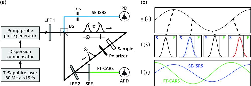
An optical schematic for DIVS is shown in Fig. 1(a). Laser pulses from a Ti:sapphire oscillator (Coherent Vitara-T-HP; 800-nm center, 100-nm bandwidth) enter a 4f dispersion compensation system consisting of an SF11 prism, concave cylindrical mirror, and spatial light modulator (SLM; Santec SLM-200). For dispersion compensation, we performed pulse shaping with a stochastic genetic algorithm that used the nonresonant FT-CARS signal from distilled water as a measure of fitness.44 The theoretical transform-limited pulse width for our laser bandwidth was 9.4 fs. Laser pulses then enter a pump–probe pulse generator comprising a zero-order half-wave plate and a Michaelson interferometer with a polarizing beamsplitter and quarter-wave plates in each arm. Inside the interferometer, the path length of the probe arm is fixed, while that of the pump arm is rapidly scanned at 12 kHz in a 4f system with a resonant scanner (Cambridge Technology CRS 12 kHz). Exiting the pump–probe pulse generator are cross-polarized pump and probe pulses with a variable optical delay (τ) scanned over a maximum ∼1.9ps of the molecular vibrational coherence at a rate of 24,000scans/s. Optical delay is accurately measured for FT-CARS and SE-ISRS signals using the interference from a 1064-nm continuous-wave laser (QPhotonics QFBGLD-1060-400) superposed on the Ti:sapphire beam throughout the pump–probe pulse generator.

Pump and probe pulses pass through a 750-nm long-pass filter (LPF 1; Edmunds #66-226) before entering a Sagnac interferometer (SI), where they are split at a beamsplitter (BS; EKSMA 042-7750SB) into clockwise (CW) and counterclockwise (CCW) paths at CW:CCW ratios of 80:20 and 50:50, respectively. While the 50:50 ratio for probe pulses provides optimal destructive interference at the SI output, the 80:20 ratio for pump pulses allows more pump light to reach the sample than in the case of a 50:50 pump split. In the CW direction, pulses are focused by an achromatic lens onto the sample, where the pump pulse excites a vibrational coherence causing an oscillatory refractive index [Fig 1(b), upper panel]. As a result, the phase of the electric field of the following transmitted probe pulse is modulated with τ dependence. The transmitted probe may be (1) frequency shifted blueward, (2) frequency shifted redward, (3) phase-delay shifted forward, or (4) phase-delay shifted backward, depending on the slope of the refractive index oscillation at the time of transmission.18^,45 After the sample, a polarizer removes the pump pulse. The probe is then filtered by a second 750-nm long-pass filter (LPF 2; Thorlabs FELH0750), which serves to spectrally separate the probe for detection of the SE-ISRS (transmitted) and FT-CARS (reflected) signals. Reflected off LPF 2, the probe passes through a 750-nm short-pass filter (SPF; Chroma ET750SP-2P-1500) and is focused by an achromatic lens onto an avalanche photodiode (APD; Thorlabs APD120A). The τ-dependent spectral shifting of the probe, which passes through the SPF, results in an intensity oscillation that is detected as the FT-CARS signal [Fig. 1(b), middle and lower panels]. The portion of the probe that passes through LPF 2 returns to the beamsplitter of the SI. Exiting the SI in the upward direction, the CW probe interferes with the CCW probe field, which functions as a local oscillator (LO; no τ-dependent phase modulation), as described in our previous work.42 The τ-dependent phase shifting of the probe and its interference with the LO results in an intensity oscillation, which is detected as the SE-ISRS signal [Fig. 1(b)]. Due to imperfections in the overlap of the probe and LO fields, the intensity at the SI output (and thus the SE-ISRS signal SNR) is spatially variant. To overcome this issue, we used an iris to select a portion of the beam which provides a high SE-ISRS SNR. The SE-ISRS beam was focused by an achromatic lens and detected by a silicon-amplified photodiode (PD; Thorlabs PDA10A-EC). The time-domain FT-CARS, SE-ISRS, and continuous-wave laser interferogram signals were all simultaneously recorded via a high-speed digitizer (Alazartech ATS9440) and computer with the included digitizer software. The LPF 1 and LPF 2 angles were set to <5deg offset from the laser beam path. The SPF angle was adjusted so as to transmit the maximum intensity of the tetrabromoethane signal (the sample with the strongest signal) before saturation of the coherence spike at the APD. The laser power at the sample was 120 mW, with a pump:probe power ratio of 1:1, which we empirically determined to be SNR-maximizing in our DIVS experiments. The probe power at the SI input was 120 mW. For the data shown in Figs. 2 and 3, the probe power at the SI output was ∼3.5mW (∼2.9% of input). For the data shown in Fig. 4 and Appendix A, the probe power at the SI output was ∼7.0mW (∼5.8%). After the iris, the probe power was typically 100 to 500μW.

Figure 2 shows time-domain signals of a bromoform–benzene mixture (1:1 volume ratio) acquired by DIVS. SE-ISRS and FT-CARS signals were detected simultaneously at a rate of 24,000spectra/s, corresponding to an acquisition time of both signals within 41.7μs. Signals shown in Fig. 2 were electronically low-pass filtered (1.9-MHz cutoff, Mini-Circuits BLP-1.9+), and their mean signal amplitudes (DC offsets) were removed. Accurate temporal scaling of each trace was performed by interpolating the raw time-domain data with the unwrapped continuous-wave laser interferogram, compensating for the nonlinear movement of the resonant scanner. Qualitatively evident from the time-domain signals is the difference between the Raman frequency-dependent sensitivities of SE-ISRS and FT-CARS.

Raman spectra were acquired by calculating the power spectra of the DIVS time-domain signals, here using a 1.58-ps region starting from 43-fs probe delay. Figure 3 shows waterfall plots of SE-ISRS [Fig. 3(a)] and FT-CARS [Fig. 3(b)] spectra of a 1:1 (volume ratio) bromoform–benzene mixture measured by DIVS at 24,000spectra/s. Spectra of pure bromoform, benzene, toluene, and tetrabromoethane are provided in Appendix A. Time-domain signals were electronically low-pass filtered (11-MHz cutoff, Mini-Circuits BLP-10.7+), their DC offsets were removed by subtracting the average voltage, and their slowly oscillating components were removed computationally by a third-order polynomial fit. Power spectra were calculated via discrete Fourier transform with zero-padding and a Hanning window function (Igor Pro 8). Figure 3 insets show 1500-spectra averages, zoomed in. Individual spectra in the waterfall plots were normalized to the average power over 2000 to 2400cm−1 (a region with no reported Raman signals) in the 1500-spectra average. As seen in Fig. 3, lower-frequency Raman modes were strongly detected in the SE-ISRS spectra though attenuated in the FT-CARS spectra. The difference is most starkly seen in the case of the 154-cm−1 (4.6 THz) mode of bromoform, which was detected in individual SE-ISRS spectra but not in those of FT-CARS. On the other hand, toward higher frequencies in the fingerprint region, FT-CARS provided superior performance compared with SE-ISRS; the 1178-cm−1 mode of benzene was detected in individual FT-CARS spectra but not in individual SE-ISRS spectra. These results illustrate the comparative advantages of the two signals with respect to the detected spectral region (low-frequency versus fingerprint) and support the merit of their simultaneous detection by DIVS.

To quantitatively compare the Raman spectral sensitivity regions of SE-ISRS and FT-CARS and further investigate simultaneous detection in DIVS, we plot the ratio of the SE-ISRS SNR over the FT-CARS SNR as a function of the detected Raman mode frequency (Fig. 4, left axis). SNR was calculated from individual spectra as SNR=PR−μ∑(xi−μ)2, where PR is the signal power at the Raman mode frequency, μ is the mean power of the noise region (background offset), and xi is the power at the i’th frequency value in the noise region. For SNR calculations, we used the Raman spectral region of 2000 to 2400cm−1 for the noise, which lies beyond the sensitivity region provided by our laser and is a noise region for all samples.46^–48 We measured four samples with the same experimental settings: (1) bromoform (BF), (2) toluene (TOL), (3) benzene (BEN), and (4) tetrabromoethane (TBE). SE-ISRS or FT-CARS SNR values used for the ratios shown in Fig. 4 were calculated as the mean of the SNR values from 15,000 individual spectra, comprising 10 discrete measurements of 1500 spectra taken at 24,000spectra/s, with the 10 measurements mutually separated in laboratory time by several seconds. To show the performance variation on a timescale of seconds (further explanation provided in Appendix A), we provide in Table 1 the standard deviation of the average SNRs of the 10 measurements. In the individual continuous measurements of 1500 spectra, the standard deviations of the SNRs of SE-ISRS and FT-CARS are typically 30% to 40% of the mean values. Further tables of SNR averages and standard deviations for SE-ISRS and FT-CARS are provided in Appendix A. The dashed line indicates equivalence in SNR with respect to both signals (Fig. 4, left axis). We did not plot modes for which the mean SNR of either SE-ISRS or FT-CARS was below 0.5.

The solid curve represents the theoretical ratio of Raman frequency-dependent SE-ISRS and FT-CARS signal powers in DIVS (Fig. 4, right axis). Derivations and further explanations of the following equations briefly describing SE-ISRS and FT-CARS are given in Appendix B. The SE-ISRS electric field at the output of the SI in the detection direction is given by ESE−ISRS(ω,τ)=HLPF2(ω)[(12+β)2EPr(ω,τ)−(12−β)2ELO(ω)],(1)where HLPF2(ω) is the spectral transfer function of transmission of LPF 2, EPr(ω,τ) is the CW probe field with τ-dependent phase modulation before LPF 2, ELO(ω) is the CCW probe field acting as a local oscillator, and β is the fraction of the electric field in addition to 1/2, which is transmitted at the beamsplitter in the SI. The SE-ISRS signal is detected by a photodiode as a time-domain interferogram given by ISE−ISRS(τ)=∫0∞|ESE−ISRS(ω,τ)|2dω. Similar to conventional SE-ISRS spectroscopy, the largest contributor to the SE-ISRS intensity oscillation in DIVS originates from the destructive interference of EPr(ω,τ) and ELO(ω). This destructive interference depends on the phase delay of EPr(ω,τ), proportional to the sample refractive index. The FT-CARS electric field after the SPF can be described as EFT−CARS(ω,τ)=HSPF(ω)EPr(ω,τ),(2)where HSPF(ω) is the spectral transfer function of transmission of the SPF. Since the spectral filtering effect of passing through the SPF is greater than that of reflecting LPF 2 (due to the difference in their cutoff wavelengths by angle setting), we ignore the effect of the latter here. The FT-CARS signal is also detected by a photodiode as a time-domain interferogram and is given as IFT−CARS(τ)=∫0∞|EFT−CARS(ω,τ)|2dω. Like in conventional FT-CARS spectroscopy, in DIVS, the FT-CARS signal comes from the τ-variant intensity of probe photons that pass through the SPF. The frequency and power of this oscillation come from the τ-dependent frequency shift of the probe and are proportional to the temporal derivative of the refractive index at the sample. In Fig. 4, we plot the ratios of SE-ISRS and FT-CARS spectral powers at single simulated Raman mode frequencies at 100-cm−1 steps over the range shown in the x-axis of the figure. Our simulation of the frequency-dependent ratio of SE-ISRS and FT-CARS signal powers is a reasonably good match to the experimental results measuring the ratio of their SNRs.

Figure 4 quantitatively shows that in DIVS, SE-ISRS has a comparatively higher SNR for Raman modes below approximately 700cm−1 including the low-frequency region, while the SNR of FT-CARS is higher above the equivalence crossover point including a majority of the fingerprint region. At the lowest mutually detected mode, the 219-cm−1 mode of tetrabromoethane, the SE-ISRS SNR was greater than that of FT-CARS by a factor of 656. At the highest mutually detected mode, the 1211-cm−1 mode of toluene, the FT-CARS SNR was greater than that of SE-ISRS by a factor of 16. The low-frequency modes of tetrabromoethane at 66 (2.0 THz), 104 (3.1 THz), and 169cm−1 (5.1 THz) and bromoform at 154cm−1 (4.6 THz) were detected in individual SE-ISRS spectra at 24,000spectra/s but could not be detected by FT-CARS. These deviations from equivalence represent a comparative loss or gain in sensitivity in the case of implementing either SE-ISRS or FT-CARS spectroscopy alone, while at the same time indicating the value of their simultaneous detection enabled by DIVS.

The strength of DIVS originates from the differing yet complementary nature of the SE-ISRS and FT-CARS signals, which are detected together. The SE-ISRS signal is proportional to the sample refractive index, while that of FT-CARS is proportional to the temporal derivative of the refractive index. With SE-ISRS, the signal power increases as the detected Raman mode decreases down to the limit defined by the maximum probe delay, around 18cm−1 in our DIVS system, below which it falls to zero. With FT-CARS, the signal power is zero at 0cm−1 and increases to a maximum value as the detected mode frequency is increased, before again diminishing to zero toward higher frequencies. The frequency at which the FT-CARS signal power is maximized, as well as the overall shape of the frequency-dependent FT-CARS power curve, is determined by the pump and probe pulse widths and the LPF 1, LPF 2, and SPF angles in DIVS. With our system, one can conveniently change the frequency-dependent sensitivity of DIVS by adjusting the angles of LPF 1 and SPF.

The high-frequency limit of DIVS (the highest detectable mode by FT-CARS) is determined either by sampling limitations of the time-domain signal (considering the spectral acquisition rate, maximum probe delay, laser repetition rate, and digitizer sampling rate) or by the bandwidth of the pulse laser after LPF 1. In our DIVS setup, we are limited by the latter, with the pulse width of our filtered laser corresponding to a Raman excitation bandwidth of <1600cm−1. With a Ti:sapphire oscillator generating shorter pulses, FT-CARS spectroscopy has been demonstrated over the range of 200 to 3600cm−1 at the same spectral acquisition rate of 24,000spectra/s.36 In principle, by simply changing the laser used in this paper to one with a broader spectrum, we can increase the high-frequency limit of DIVS. The low-frequency limit (the lowest detectable mode by SE-ISRS, also equal to the Raman spectral resolution) is determined by the maximum probe delay. In our setup, the maximum delay of ∼1.9ps is limited by the maximum displacement of the resonant scanner mirror. In principle, this could be increased to 8 ps by switching to a polygonal mirror-based delay scanning technique similar to that previously demonstrated with FT-CARS spectroscopy performed at 50,000spectra/s,37 which would improve the low-frequency limit and spectral resolution to 4.2cm−1. This change would also increase the spectral acquisition rate in DIVS, limited in our system by the speed of mechanical scanning of the probe delay. In principle, DIVS is also fully compatible with the faster method of pump–probe group delay scanning used in quasi-dual-comb CARS spectroscopy41 (100,000spectra/s).

As described in Sec. 3.3, Appendix B, and our previous work,42 the SNR of SE-ISRS depends on the probe background reduction provided by the destructive interference of the CW and CCW fields. In our current DIVS setup, the destructive interference at the SI output is spatially nonuniform, leading to a spatially variant SE-ISRS SNR. In this work, we addressed the problem simply by using an iris to select a particular region of the SE-ISRS beam before detection. However, this is an inefficient solution; the full probe beam profile representing the entire potential SE-ISRS signal is truncated spatially by >90%. We believe one cause of the spatially nonuniform probe beam is a distorted wavefront at the SI input. By transmission through the optical components in the SI at different timings, differences between the CW and CCW wavefronts are exacerbated, resulting in imperfect interference at the SI output, which cannot be easily overcome by system alignment. Improving the uniformity of the probe wavefront at the SI input could potentially address this issue to some degree, ultimately improving the SE-ISRS SNR.

In this paper, we have presented DIVS, a technique for coherent Raman spectroscopy which allows simultaneous detection of SE-ISRS and FT-CARS at a spectral acquisition rate of 24,000spectra/s. Our proof-of-concept measurements of four liquid solvents with Raman modes covering the range of 66 (2.1 THz) to 1211cm−1 demonstrate the ability of DIVS to perform broadband measurements of the low-frequency and fingerprint regions simultaneously and rapidly. We quantitatively compared the two signals by plotting the ratio of their SNRs as a function of the detected Raman mode, showing their comparative strengths and thus the merit of simultaneous detection enabled by DIVS. In our demonstration of DIVS, the SE-ISRS signal showed a >500× enhancement of SNR below 200cm−1 (6.5 THz) compared with that of FT-CARS, and the FT-CARS signal showed a >10× enhancement of fingerprint SNR above 1000cm−1 compared with that of SE-ISRS. Considering the early stage of the method, DIVS may be a useful technique for temporally resolved measurements of pure or high-concentration samples that have significant vibrational information in both the THz and fingerprint regions. One direction might be toward the field of material science, with potential applications in investigating polymers, which often have rich information in the fingerprint and low-frequency regions.16^,49

To demonstrate the capability of DIVS for ultrafast broadband Raman spectroscopy over the THz and fingerprint regions, we measured the Raman spectra of four liquid chemicals at 24,000spectra/s: bromoform, benzene, toluene, and tetrabromoethane. In this Appendix A, we report the results of these experiments in more detail than what is provided in the main text. Mean SNR values below 0.5 were excluded.

Here, we show waterfall plots of SE-ISRS and FT-CARS spectra of bromoform (Fig. 5) and benzene (Fig. 6) acquired by DIVS at 24,000spectra/s. Analogous to Fig. 3, insets show the 1500-spectra averages. Table 2 shows the average SNR values from individual FT-CARS and SE-ISRS spectra of bromoform and benzene acquired by DIVS. As in the main text above, the data here were calculated by averaging the mean SNRs of 1500 spectra across 10 experiments per pure sample (equivalent to the mean SNR of 15,000 spectra). Standard deviations calculated from the 10 SNR averages are also provided (n=10). Evident from these and the following data of other samples, the coefficient of variation (the ratio of the standard deviation to the mean) was overall greater in the case of SE-ISRS (0.025 to 0.095 for mean SNR>5) than in the case of FT-CARS (0.008 to 0.023 for mean SNR>5). We believe this was due to fluctuations of the SI alignment caused by laboratory air currents and other vibrations (i.e., on a long timescale), which affect the probe background extinction at the SI output and thus the SNR of SE-ISRS. This is in contrast to the standard deviation of the SE-ISRS and FT-CARS SNRs in a given continuous 1500-spectra measurement (i.e., on a short timescale). In these cases, the coefficients of variation for SE-ISRS and FT-CARS were 0.30 to 0.38 and 0.38 to 0.40, respectively. At this time, we cannot explain this result. To mitigate the SE-ISRS SNR fluctuation on slow timescales caused by air currents, the authors suggest using a physical shield around the Sagnac interferometer (which was not employed in this study).

In Fig. 7, we show waterfall plots of SE-ISRS and FT-CARS spectra of toluene, acquired by DIVS at 24,000spectra/s. Table 3 shows the average SNRs from individual spectra, in a manner similar to Table 2. In the averaged SE-ISRS spectra of these results, we did not observe strong low-frequency mode enhancement of the depolarized 216-cm−1 mode (b2) of toluene47 compared with the averaged FT-CARS spectra. In these data, the FT-CARS SNR of this mode was 5.7× greater than that of SE-ISRS. This was a highly unexpected result, considering our theoretical model as well as the experimental 1108×, 233×, and 255× enhancements of the SE-ISRS spectral average SNR over that of FT-CARS for the neighboring 169- (tetrabromoethane, depolarized), 219- (tetrabromoethane, polarized), and 223-cm−1 (bromoform, polarized) modes, respectively. If the 216-cm−1 mode of toluene was to match our expectation of a >200× ratio of SE-ISRS SNR to FT-CARS SNR in the spectral averages, our experimental results represent a value that differs from expectation by more than three orders of magnitude. Other modes of toluene follow the empirical trend and theoretical curve shown in Fig. 4. At this time, we cannot explain this result.

In Fig. 8, we show waterfall plots of SE-ISRS and FT-CARS spectra of tetrabromoethane, acquired by DIVS at 24,000spectra/s. Analogous to Fig. 3, insets show the 1500-spectra averages. Table 4 shows the average SNRs from individual spectra, similar to Table 1.

To investigate the concentration-dependent sensitivity of DIVS, we performed measurements of liquid solvent samples mixed in varying concentrations. Specifically, we used DIVS to measure the signals of bromoform and benzene in 99.5% ethanol at concentrations of 5 M, 2.5 M, 1 M, 500 mM, and 250 mM (1 M = 1 mol/L; Fig. 9). After preparation, samples were immediately sealed and measured within 15 min. SNR values were calculated as the average of the SNRs from 15,000 spectra (1500 spectra over 10 measurements). As shown in Fig. 9, the signals from strong modes of benzene and bromoform were detected at 24,000 spectra/s at concentrations as low as 500 mM.

To further understand the detected SE-ISRS and FT-CARS signals in DIVS, we formulate their mathematical expressions below, following previous descriptions of ISRS18 and SE-ISRS.42 The probe pulse passes through LPF 1 and is described as E˜LPF1(t)=F−1[HLPF1(ω)S(ω)],(3)where F−1[*] is an inverse Fourier transform, HLPF1(ω) is the spectral transfer function of LPF 1, and S(ω) is the probe spectral amplitude before LPF 1. The probe is then split at the entry of the SI at a 50:50 beamsplitter into CW and CCW directions. In the CW direction following the pump after delay τ, the probe phase is modulated according to the oscillatory refractive index at the sample, synchronized with molecular vibrations. The probe field after passing through the sample is described as E˜Pr(t,τ)=e−iωc[n(t,τ)+n2|E˜LPF1(t)|2]zcE˜LPF1(t),(4)where the term exp{−iωc[n(t,τ)+n2|E˜LPF1(t)|2]zc} describes the τ-dependent probe phase modulation and probe self-phase modulation after transmission of the sample, and n(t,τ), n2, z, and c are the τ-dependent refractive index, second-order refractive index, sample path length in m, and speed of light in m/s, respectively. The τ-dependent refractive index is described as n(t,τ)=n0{1+∑kNAke−(t+τ)γksin[ωk(t+τ)]},(5)where n0 is the refractive index of the sample at equilibrium, and Ak, ωk, and γk are the k’th Raman mode amplitude, angular frequency, and damping constant, respectively. While the term n(t,τ) results in probe phase oscillation corresponding to molecular vibrations, the term n2|E˜LPF1(t)|2 generates a non-resonant probe background, which can function as a local oscillator in FT-CARS.50 We assume here that differences between the self-phase modulations of the CW and CCW probes in SE-ISRS are negligible, and, due to destructive interference at the SI output as well as a far larger residual probe background, the generated nonresonant background plays a comparatively minor role in SE-ISRS. After passing through the polarizer, the probe is spectrally filtered by LPF 2. The portion reflected at LPF 2 that passes through the SPF is detected as the FT-CARS time-domain signal, described as IFT−CARS(τ)=∫0∞|HSPF(ω)EPr(ω,τ)|2dω,(6)where HSPF(ω) is the spectral transfer function of the SPF. In our setup, SPF and LPF 2 have redundant effects on the FT-CARS signal, and we ignore the latter’s effects in Eq. (6).

In the case of SE-ISRS, transmission of LPF 2 has a minor filtering effect on the CW probe, and we describe its electric field returning to the beamsplitter as E˜CW(t,τ)=F−1[HLPF2(ω)EPr(ω,τ)],(7)where HLPF2(ω) is the spectral transfer function of LPF 2. In the CCW direction, the probe is filtered by LPF 2 and passes through the sample without a preceding pump pulse. Without an oscillatory refractive index at the sample, the CCW probe field reaches the beamsplitter and is described as E˜CCW(t)=F−1[F[e−iωc[n0+n2|E˜LPF1(t)|2]zce−iδF−1[HLPF2(ω)HLPF1(ω)S(ω)]]],(8)where F[*] is a Fourier transform, and δ represents a fixed phase offset relative to E˜CW(t,τ). At the output of the SI in the upward direction, the CW and CCW probe fields interfere, the τ-dependent intensity of which is detected as the SE-ISRS time-domain signal, formulated as ISE−ISRS(τ)=∫0∞|F[(12+β)2E˜CW(t,τ)−(12−β)2E˜CCW(t)]|2dω,(9)where β is the fraction of the probe field beyond 1/2, which passes through the beamsplitter of the SI. In our simplified description of the SE-ISRS electric field in the main text, we assumed that the effect of LPF 2 (1) is the same for the CW and CCW probe fields and (2) can be treated as if LPF 2 was placed at the SI output.

The theoretical curve plotted in Fig. 4 was calculated from simulations of SE-ISRS and FT-CARS in DIVS, using Eqs. (6) and (9) above. For simulations, we assumed a Gaussian spectral profile for the probe with a center wavelength and full width at half maximum of 800 and 100 nm, respectively. β=0.12, Ak=1×10−5, γk=0.36×1012s−1, n0=1.54, n2=2.2×10−13cm2/W, z=1.0×10−4m, and δ=1. The peak intensity of E˜LPF1(t) is assumed to be 3×109W/cm2. The maximum probe delay was 1.5 ps. Spectral transmission profiles of the filters were obtained from the manufacturers, and their specifications were approximated using built-in filtering functions in Igor Pro 8. For LPF 1 and LPF 2, we calculated an LPF with 300 coefficients, a Hamming window function, pass band at 3.9977×1014Hz, and reject band at 4.017×1014Hz. For SPF, we calculated an SPF with 800 coefficients, a Hanning window function, pass band at 4.042×1014Hz, and reject band at 4.082×1014Hz. The time-domain signals of SE-ISRS and FT-CARS were normalized to their respective average probe intensities, and the DC offsets were subtracted. For the final plotted curve, the SE-ISRS power was increased by a factor of 67 to align the equivalence crossover point with the apparent same point in the experimental data.

For additional clarity, we also plot in Fig. 10 the simulated signal powers of FT-CARS and SE-ISRS in DIVS, according to the equations and simulation parameters presented above. Note that here we do not consider sensitivity limitations imposed by the pump bandwidth. In our system, the pump pulse bandwidth causes attenuation of both DIVS signal powers above 1600cm−1. For further insight into impulsive vibrational spectroscopy including the effects of the pump bandwidth on the signal power, we refer readers to a recent review on low-frequency coherent Raman spectroscopy by Bartels et al.51

Walker Peterson is a PhD candidate in the Department of Chemistry of the University of Tokyo. He received his BA degree in music (summa cum laude) and chemistry (magna cum laude) from Amherst College in 2011. He received his MS degree in physical chemistry from the University of Tokyo in 2019. He is currently a student member of SPIE and was a founding member and president of the UTokyo Student Chapter.

Julia Gala de Pablo is a Japan Society for the Promotion of Science (JSPS) postdoctoral fellow in the Department of Chemistry of the University of Tokyo. She received her BSc degree in physics and biochemistry from the University Complutense of Madrid in 2014 and 2015, respectively. She received her PhD in physics from the University of Leeds in 2019.

Matthew Lindley is a PhD candidate in the Department of Chemistry of the University of Tokyo and holds a DC fellowship from the JSPS. His work focuses on nonlinear optical flow cytometry.

Kotaro Hiramatsu is an assistant professor in the Department of Chemistry and the Research Center for Spectral Chemistry of the University of Tokyo and an adjunct researcher of the Precursory Research for Embryonic Science and Technology Program of Japan Science and Technology Agency. He received his PhD in chemistry from the University of Tokyo, Japan, in 2016.

Keisuke Goda is a professor in the Department of Chemistry of the University of Tokyo, an adjunct professor in the Department of Bioengineering of the University of California, Los Angeles (UCLA), and an adjunct professor at the Institute of Technological Sciences of Wuhan University. His research group aims to develop serendipity-enabling technologies based on laser-based molecular imaging and spectroscopy, together with microfluidics and computational analytics, and use them to push the frontiers of human knowledge.