• Photonics Research
  • Vol. 6, Issue 8, A43 (2018)
Constantinos Valagiannopoulos* and Vassilios Kovanis
Author Affiliations
  • Department of Physics, School of Science and Technology, Nazarbayev University, 53 Qabanbay Batyr Ave, Astana KZ-010000, Kazakhstan
  • show less
    DOI: 10.1364/PRJ.6.000A43 Cite this Article Set citation alerts
    Constantinos Valagiannopoulos, Vassilios Kovanis. Engineering the emission of laser arrays to nullify the jamming from passive obstacles[J]. Photonics Research, 2018, 6(8): A43 Copy Citation Text show less
    Schematic of the regarded configuration. The aggregate field of an active laser array is perturbed by a passive cylindrical obstacle.
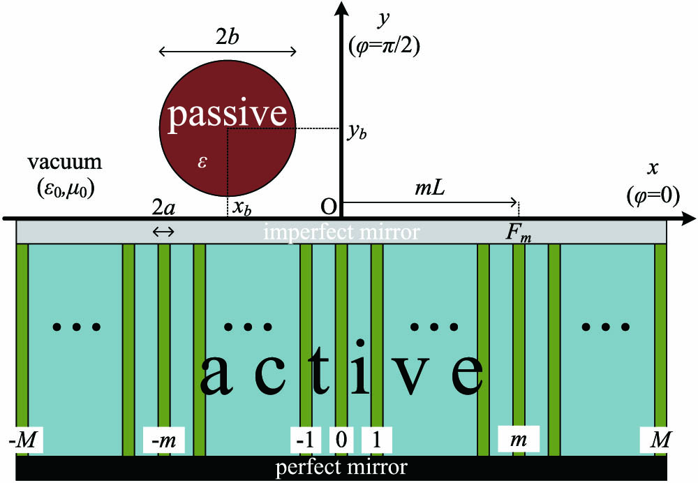
    Fig. 1. Schematic of the regarded configuration. The aggregate field of an active laser array is perturbed by a passive cylindrical obstacle.
    Percent error of the obstacle-free optimal solution as functions of: (a) radius of the obstacle b/λ0 (ϵ=2) and (b) relative permittivity of the obstacle ϵ (b=λ0/4) for several vertical positions yb. Plot parameters: G˜(φ)=e−γ(φ−ϑ)2, ϑ=90°, γ=10, k0L=0.1, M=80, U=12, xb=0.
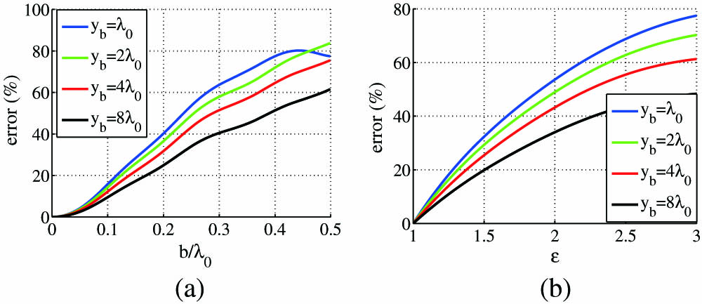
    Fig. 2. Percent error of the obstacle-free optimal solution as functions of: (a) radius of the obstacle b/λ0 (ϵ=2) and (b) relative permittivity of the obstacle ϵ (b=λ0/4) for several vertical positions yb. Plot parameters: G˜(φ)=eγ(φϑ)2, ϑ=90°, γ=10, k0L=0.1, M=80, U=12, xb=0.
    Percent error of the obstacle-free optimal solution as a function of the horizontal position of the obstacle xb/D=xb/(ML) for several (a) radii b/λ0 (ϵ=2) and (b) permittivities ϵ (b=λ0/4). Plot parameters: yb=2λ0, and the remaining ones the same as in Fig. 2.
    Fig. 3. Percent error of the obstacle-free optimal solution as a function of the horizontal position of the obstacle xb/D=xb/(ML) for several (a) radii b/λ0 (ϵ=2) and (b) permittivities ϵ (b=λ0/4). Plot parameters: yb=2λ0, and the remaining ones the same as in Fig. 2.
    Percent error of the obstacle-free optimal solution in contour plot of the permittivity ϵ and the electrical radius of the cylinder b/λ0 for (a) centered obstacle (xb=0) and (b) off-centered obstacle (xb=ML=D=4λ0/π). Plot parameters: yb=2λ0 and the remaining ones the same as in Fig. 2.
    Fig. 4. Percent error of the obstacle-free optimal solution in contour plot of the permittivity ϵ and the electrical radius of the cylinder b/λ0 for (a) centered obstacle (xb=0) and (b) off-centered obstacle (xb=ML=D=4λ0/π). Plot parameters: yb=2λ0 and the remaining ones the same as in Fig. 2.
    Ideal target G˜(φ) and the optimal actual pattern G(φ) (both real and imaginary parts) as functions of azimuthal angle φ for the obstacle-free solution of Ref. [5] with (a) b=λ0/8, (b) b=λ0/4, (c) b=λ0/2, and (d) for the solution of Section 2 of this study and the worst case b=λ0/2. Plot parameters: ϵ=2, xb=0, yb=2λ0, and the remaining ones the same as in Fig. 2.
    Fig. 5. Ideal target G˜(φ) and the optimal actual pattern G(φ) (both real and imaginary parts) as functions of azimuthal angle φ for the obstacle-free solution of Ref. [5] with (a) b=λ0/8, (b) b=λ0/4, (c) b=λ0/2, and (d) for the solution of Section 2 of this study and the worst case b=λ0/2. Plot parameters: ϵ=2, xb=0, yb=2λ0, and the remaining ones the same as in Fig. 2.
    (a) Percent error of optimal solution without and with the obstacle as a function of the optical distance between two neighboring lasers k0L. (b) Ideal target G˜(φ) and the optimal actual pattern G(φ) (both real and imaginary parts) as functions of azimuthal angle φ for k0L=2.4. The configuration of Fig. 5(c) is considered.
    Fig. 6. (a) Percent error of optimal solution without and with the obstacle as a function of the optical distance between two neighboring lasers k0L. (b) Ideal target G˜(φ) and the optimal actual pattern G(φ) (both real and imaginary parts) as functions of azimuthal angle φ for k0L=2.4. The configuration of Fig. 5(c) is considered.
    Ideal target G˜(φ) and the optimal actual pattern G(φ) (both real and imaginary parts) as functions of azimuthal angle φ for the obstacle-free solution of Ref. [5] with (a) ϵ=1.5, (b) ϵ=2, (c) ϵ=2.5, and (d) for the solution of Section 2 of this study and the worst case ϵ=2.5. Plot parameters: G˜(φ)=e−βφ[1+A cos(αφ)], A=0.7, α=13.5, β=0.2, k0L=1, M=50, U=12, b=λ0/4, xb=0, yb=2λ0.
    Fig. 7. Ideal target G˜(φ) and the optimal actual pattern G(φ) (both real and imaginary parts) as functions of azimuthal angle φ for the obstacle-free solution of Ref. [5] with (a) ϵ=1.5, (b) ϵ=2, (c) ϵ=2.5, and (d) for the solution of Section 2 of this study and the worst case ϵ=2.5. Plot parameters: G˜(φ)=eβφ[1+Acos(αφ)], A=0.7, α=13.5, β=0.2, k0L=1, M=50, U=12, b=λ0/4, xb=0, yb=2λ0.
    Block diagram for the introduced processes and presented concepts of the study at hand. A greedy inverse search by trial and error for the actual obstacle; as long as the error is non-negligible, a new trial object is considered.
    Fig. 8. Block diagram for the introduced processes and presented concepts of the study at hand. A greedy inverse search by trial and error for the actual obstacle; as long as the error is non-negligible, a new trial object is considered.
    Constantinos Valagiannopoulos, Vassilios Kovanis. Engineering the emission of laser arrays to nullify the jamming from passive obstacles[J]. Photonics Research, 2018, 6(8): A43
    Download Citation