
Chaojun Niu, Fang Lu, Xiang'e Han. Propagation Properties of Gaussian Array Beams Transmitted in Oceanic Turbulence Simulated by Phase Screen Method[J]. Acta Optica Sinica, 2018, 38(6): 0601004
- Acta Optica Sinica
- Vol. 38, Issue 6, 0601004 (2018)
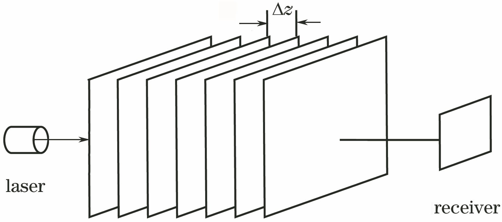
Fig. 1. Sketch map of multi-layer phase screen method
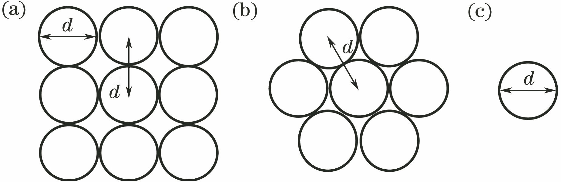
Fig. 2. Schematic of different beam arrangements. (a) 3×3 beam array with rectangle distribution; (b) 7 beam array with radial distribution; (c) single Gaussian beam
Fig. 3. Average radii of beams under different turbulence conditions. (a) Z=10 m, ε=10-6 m2·s-3, ω=-2,η=0.001 m, λ=532 nm; (b) Z=10 m, ε=10-6 m2·s-3, χT=10-6 K2·s-1, η=0.001 m, λ=532 nm; (c) ε=10-6 m2·s-3, χT=10-6 K2·s-1, ω=-2, η=0.001 m, λ=532 nm; (d) Z=10 m, χT=10-6 K2·s-1, ω=-2, η=0.001 m, λ=532 nm
Fig. 4. Distribution of spot centroid
Fig. 5. Standard deviation of spot centroid wander. (a) Z=10 m, ε=10-6 m2·s-3, ω=-2, η=0.001 m, λ=532 nm; (b) Z=10 m, ε=10-6 m2·s-3, χT=10-6 K2·s-1, η=0.001 m, λ=532 nm; (c) ε=10-6 m2·s-3, χT=10-6 K2·s-1, ω=-2, η=0.001 m, λ=532 nm; (d) Z=10 m, χT=10-6 K2·s-1, ω=-2, η=0.001 m, λ=532 nm
Fig. 6. Numerical simulation of on-axis scintillation index of beam array. (a) Z=10 m, ε=10-6 m2·s-3, ω=-2, η=0.001 m, λ=532 nm; (b) Z=10 m, ε=10-6 m2·s-3, χT=10-6 K2·s-1, η=0.001 m, λ=532 nm; (c) ε=10-6 m2·s-3, χT=10-6 K2·s-1, ω=-2, η=0.001 m, λ=532 nm; (d) Z=10 m, χT=10-6 K2·s-1, ω=-2, η=0.001 m, λ=532 nm

Set citation alerts for the article
Please enter your email address
© Copyright 2018-2021 | Chinese Laser Press. All Rights Reserved 沪ICP备15018463号-20