According to the prediction of the International Data Cooperation (IDC) in 2018, global data will increase to 175 ZB by 2025 and 2142 ZB by 2035¹. Handling this enormous increasing volume of data based on the current data storage techniques is challenging. Compared with conventional storage devices such as the flash, hard disk drive (HDD), and magnetic tape, the optical storage techniques and devices such as blue-ray optical discs², optical glass storage^{3, 4}, and HDS^5-8 feature more advantageous properties such as lower energy consumption, stable storage, and longer lifetime that can be leveraged for the long-term storage of big data. HDS handles digital information as a two-dimensional (2D) array called a data page and records a three-dimensional (3D) hologram in light-sensitive media^{6, 7, 9}. The storage density is determined by the hologram size, number of multiplexing recordings, and single data page capacity. Conventional HDS uses a binary amplitude data page^{7, 9-11}, and the capacity of a single page is limited. With the development of optical devices such as spatial light modulators (SLMs), multi-level phase-modulated HDS^12-15 and complex-amplitude-modulated HDS^16-18 that use the phase of light to encode information, have been proposed to increase the amount of information in one data page. Although phase encoding can improve the storage capacity significantly, the phase information cannot be read directly. It needs to be computationally retrieved from the intensity image captured by a detector. To demodulate the complex amplitude quickly and accurately with a simple and stable system is the key for the HDS system to keep the data transmitting rate (phase modulation is considered a special case of complex amplitude modulation with a uniform amplitude of 1).

Some researchers have attempted to decode the HDS complex amplitudes via different methods. Depending on whether there is interference in the retrieval process, HDS data demodulation systems can be divided into two types: interferometric and non-interferometric. Nobukawa proposed a complex-amplitude data page demodulation method based on digital holography and realized two-level amplitude and four-level phase demodulation¹⁶. Katano used two convolutional neural networks (CNNs) to retrieve the amplitude and phase from four interferometric holograms¹⁷. Both these methods require a reference beam, and the reading system is complicated and sensitive to environmental vibrations. Moreover, the multi-capture operation also decreases the data transfer rate. Lin proposed non-interferometric phase demodulation based on an iterative Fourier transform algorithm^{12, 19}. The optical system is simplified, but the data transfer rate decreases because of the iterative calculation in the retrieval process. Bunsen used the TIE algorithm to retrieve the complex amplitude from three diffraction intensity images¹⁸. It requires three intensity images and iteration calculations that also decrease the transfer rate. Horisaki presented a method for single shot, complex-amplitude imaging that can retrieve the phase and amplitude from a single intensity image directly. However, it is only used in handwritten digit recognition, where the distributions are relatively simple²⁰. The data reading of HDS requires a simple system to ensure both stable data transmission and fewer iterations to improve the data transfer rate. In conventional methods, it is difficult to achieve a balance between the transmission speed and stability.

In recent years, we have witnessed the emergence of deep learning that demonstrates great potential in various fields such as computer vision²¹, optical encryption²², and optical computing²³. Since the pioneering work of Sinha et al.²⁴ on the recovery of phase directly from a single diffraction intensity image, deep learning networks have been used to reconstruct the amplitude and phase directly from a hologram^25-27 or combined with physics prior to retrieving the phase from a diffraction intensity image²⁸. One can refer to a recent survey²⁹ for more details. In the existing studies, the retrieval of the complex amplitude from the hologram still needs reference beam. The system is complicated and not suitable for HDS. Physical prior-based phase retrieval from diffraction intensity does not need reference beam but requires thousands of iterations to achieve phase demodulation. Inspired by these studies, our previous work proposed a non-iterative lensless phase demodulation method based on deep learning and embedded data used in HDS³⁰. In this study, we further propose a complex amplitude encoding and demodulation method. A complex amplitude encoding method with a higher capacity is designed, and a lensless non-interferometric complex amplitude retrieval system is established. The inverse problem is decomposed into two backward operators related to amplitude and phase and represented by two CNNs separately. The four-level complex amplitude can be demodulated directly without interferometry and iteration. The experiment verifies its feasibility and demonstrates the potential of complex amplitude demodulation from a single intensity image. The analysis of the diffraction features and encoded data pages provide guidance for future research on deep learning-based complex amplitude retrieval.

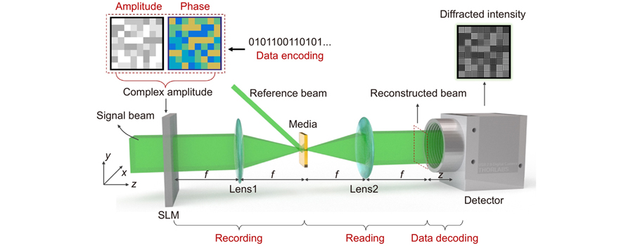
A schematic of complex amplitude modulated HDS is shown in Fig. 1. Information storage and reading in HDS include four processes: encoding, recording, reading, and decoding. In the encoding process, information is encoded into amplitude and phase data pages to modulate the signal beam. In the recording process, the signal beam is converged by Lens 1, and it subsequently interferes with a reference beam. The interference hologram is recorded in the media. In the reading process, a reconstructed beam is obtained at the focal plane of Lens 2 by using a same reference beam to irradiate the media. The reconstructed beam contains the encoded amplitude and phase information. In the decoding process, a detector is placed at distance z from the reconstructed beam plane to capture the diffraction intensity image. The complex-amplitude information is retrieved from the intensity image by the method proposed in this paper. The diffraction intensity image is used for complex amplitude demodulation, which is captured directly without any lens, so it is called a lensless complex amplitude decoding system.

According to the theory of HDS, the wavefront of the reconstructed beam is exactly the same with the recorded signal beam if the influence of the system and material noise is ignored. Information reading is to obtain the encoded amplitude and phase pages from a single-intensity image captured by the detector. The light field of the reconstructed beam is defined by Eq. (1):

1U(x,y;0)=A(x,y;0)exp(iφ(x,y;0)).

The position of the reconstructed beam plane (the back focal of Lens 2 in Fig. 1) is defined as z= 0. The diffraction field of U(x, y; z) over distance z is given by Eq. (2):

2U(x,y;z)=∫∫−∞∞F(fX,fY;0)Gexp(i2π(fXx+fYy))dfXdfY,

where G is the transfer function G=exp[i2πλ1−(λfX)2−(λfY)2z], f_X and f_Y are the spatial frequencies in the x and y directions, respectively, and F(f_X, f_Y; 0) is the angular spectrum of U(x, y, 0) , that is the Fourier transform of U(x, y, 0) shown in Eq. (3):

3F(fX,fY;0)=∫∫−∞∞U(x,y;0)exp(i2π(fXx+fYy))dxdy.

The intensity of the light field at distance z is expressed by Eq. (4):

4I(x,y;z)=|U(x,y;z)|2=H(U(x,y;0)).

Because of diffraction, the intensity I(x, y; z) recorded by the detector has a certain pattern, as shown in Fig. 1. The operator H(·) denotes the mapping function that relates the complex amplitude U(x, y; 0) and intensity image I(x, y, z).

According to the Huygens–Fresnel diffraction principle, the constructive and destructive interference of coherent light caused by diffraction produces an intensity pattern in the irradiance result I(x, y; z)³¹. A simple theoretical model was developed (Fig. 2) to describe the diffraction process in HDS demodulation. In this model, each data point on the SLM is regarded as a divergent point light source. As light propagates forward, the secondary sources corresponding to different data points are superimposed on each other to form a new light field. The further the propagation, the stronger the diffraction effect. An appropriate distance z=d can be found, where the intensity I related to a data point P is mainly determined by the eight surrounding data points (P_p,p = 1,⋯, 8). Because of the amplitude and phase difference between data points P and P_p, there is a diffraction pattern that has a clear correlation with the encoded amplitude and phase data. Both the original amplitude features and the new feature resulting from the phase difference are included in this diffraction pattern.

In order to analyze the relationship between the diffraction pattern and the amplitude-phase data numerically, we set the complex amplitude data as four-level phase (π/6, 2π/3, π, 3π/2) and amplitude (0.7, 0.8, 0.9, 1) randomly. The phase values are randomly selected from [0, 2π] at unequal intervals. It is different from the traditional encoding rule in HDS, which will be explained in the second half of this Section. The complex amplitude encoding page and intensity image are shown in Fig. 3(I). Phase-only encoding and amplitude-only encoding are also shown in Fig. 3(II) and Fig. 3(III), respectively, to facilitate the analysis of the diffraction pattern features. The diffraction distance z = 2 mm. The cross-section at the position of the red line in the intensity images is shown in Fig. 3(j). The intensity image in Fig. 3(I) shows that the complex-amplitude-based pattern consists of both the amplitude-related and phase-related features. The phase-related feature is manifest in the intensity distribution resulting from light propagation, as shown in Fig. 3(II). The amplitude-related feature in Fig. 3(III) is the original amplitude distribution that is still distinguishable under the condition of this diffraction distance.

Figure 4(a) and Fig. 4(b) is the 2D and 3D contour map of the intensity in Fig. 3(c), respectively. Fig. 4(c) is the cross-section of the red line in Fig. 4(a). Corresponding to the four data points, four diffraction regions are generated. The mean diffracted intensity of each data region in Fig. 4(c) is consistent with the amplitude distribution. Within each data point region, the intensity variation due to diffraction is a phase-dependent feature. Therefore, it is feasible to detect the amplitude and phase features separately. Here, the amplitude-related features in the diffraction intensity are clearly visible and directly related to the original amplitude. The relationship between the phase-related features and the diffraction pattern requires further analysis.

Based on the simplified theoretical model in Fig. 2, {(P,Pp),p=1,2,…,8} is defined as a symbol that consists of one central data point P and its eight adjacent data points Pp. If only the phase is considered, then the symbol is simplified as {(ϕ,ϕp),p=1,2,…,8}. Several examples of different symbols are shown in Fig. 5(I). Figure 5(II) are the corresponding diffraction intensity images. The general architecture of a symbol consisting of 3 × 3 data points is shown in Fig. 5(k). Fig. 5(l) is the intensity profile on the red line in the intensity distribution Fig. 5(f–j). Two rules can be observed in Fig. 5. First, the diffraction pattern characteristics are decided by the phase difference Δϕp between the central data point ϕ and its adjacent points ϕp. Second, the diffraction pattern characteristics are not directly decided by the absolute value of the central point ϕ. To build the relationship between the diffraction intensity and central phase value ϕ, the relationship between the diffraction feature and symbol is important.

Therefore, when designing the phase encoding rule for HDS, the phase difference should be paid more attention to. With n-level phase encoding rule {ϕi,i=1,2,⋯,n}，each phase value can be represented by a symbol set {Sϕ=ϕi,i=1,2,⋯,n}. The symbol set Sϕ=ϕi={(Δϕp|(ϕ=ϕi)),p=1,2,⋯,8,i=1,2,⋯,n} consists of 8ⁿ symbols with the architecture as shown in Fig. 5(k). The ϕ=ϕi means the central data point value in the symbols. Δϕp=ϕp−ϕ is the phase difference between the central data point and its adjacent data points. For each phase data point, the diffraction patterns are determined by the structure of the related symbols. To infer the phase ϕi of a central data point from the intensity image, the corresponding symbols in the set Sϕ=ϕi should be distinguishable. This implies that Δϕp in each symbol set Sϕ=ϕi should be different.

As an example, we analyzed and compared the four-level phase encoding (0, π/2, π, 3π/2) of conventional phase-modulated HDS^{15, 16} and (π/6, 2π/3, π, 3π/2) in this study. The phase difference Δϕp under these two encoding rules are summarized in Table 1 and Table 3. All values of Δϕp were set to [–π, π]. Meanwhile, we summarized the number of symbols in each symbol set Sϕ=ϕi and calculated the repetition probability defined as:

5Pij=NijNi,

where Nij is the number of symbols that belong to both Sϕ=ϕi and Sϕ=ϕj, and Ni is the total number of symbols in a set, Ni=n8. The repetition probabilities associated with the two encoding rules are shown in Table 2 and Table 4.

From Table 1, it can be seen that for each encoded value ϕ=ϕi, the possible generated phase differences Δϕp are same. This means that under the encoding rule (0, π/2, π, 3π/2), all symbols in set Sϕ=ϕi={Δϕp|(ϕ=ϕi),p=1,2,…,8,i=1,2,…,n} of different central phase values ϕ=ϕi are absolutely the same. The repetition probabilities Pij of all symbols in set Sϕ=ϕi and Sϕ=ϕj are 100%, as shown in Table 2. This implies that under the encoding rule (0, π/2, π, 3π/2), the diffraction patterns corresponding to different ϕi are the same, so the phase value ϕi cannot be inferred from the pattern of the diffraction intensity. For comparison, under the encoding rule (π/6, 2π/3, π, 3π/2), the phase difference Δϕp becomes distinguishable, as shown in Table 3. Therefore, the repetition probabilities of the symbol set in Table 4 are also significantly reduced. It is possible to establish a relationship between the diffraction intensity pattern and the phase value ϕ=ϕi.

This assumption was verified by the method introduced in Section Deep learning-based complex amplitude demodulation. A simulated experiment was conducted to generate datasets under two encoding rules (0, π/2, π, 3π/2) and (π/6, 2π/3, π, 3π/2). Two CNNs were used to detect patterns in diffracted intensity images and establish relationships with amplitude and phase data pages, respectively. The core of the CNN is the convolution kernel, which is used to extract features of different scales in the input image. The hyperparameters of the CNN is set same as the experiment discussed in Section Experiments. During the training, the mean square error (MSE) losses represents the gap between the predicted and the true value of the two cases are shown in Fig. 6(a) and Fig. 6(b). The red and black lines represent the losses for the test and training sets, respectively. The smaller the loss function value, the closer the predicted result is to the ground truth value. A detailed description of the neural network geometry and training is provided in Section Deep learning-based complex amplitude demodulation and Experiments. As shown in Fig. 6(a), the loss function values of the training and test sets do not converge after a brief plunge as the training progresses. Upon continued training, the training loss began to decrease, whereas the test loss increased, indicating that the model training resulted in overfitting. Under the encoding rule (0, π/2, π, 3π/2), the model failed to establish the relationship between the diffraction intensity and phase data page. However, as shown in Fig. 6(b), as the training progresses, the losses of both the training and test sets drop rapidly and approach zero. This implies that the CNN can not only fit the data of the training set appropriately, but can also be generalized to the test set. In other words, the deep learning model can correctly represent the relationship between the diffraction intensity and phase data page under the encoding rule of (π/6, 2π/3, π, 3π/2).

The results in Tables 1–4 and Fig. 6 show the significant difference in phase encoding between the conventional iterative method based on physical processes^{15, 16, 32} and the data-driven deep learning method in this study. In this study, we only compare two encoding rules and explain why the conventional encoding is not suitable for our deep learning method. It is worth emphasizing that the encoding rule (π/6, 2π/3, π, 3π/2) is feasible, but is not necessarily the optimal rule. In fact, the optimal encoding rules for lensless phase retrieval methods require further research which is beyond the scope of the present study.

From the analysis in Section Complex amplitude encoding and Fresnel diffraction, the amplitude and phase can be related to different features of the diffraction intensity. Therefore, operator H−1(⋅) in Eq. (4) can be split into two operators, HA−1(⋅) and Hφ−1(⋅), as shown in Eq. (6).

6A(u,v)=HA−1(I(u,v)),ϕ(u,v)=Hϕ−1(I(u,v)),

where A(u,v) is the amplitude data page, and ϕ(u,v) is the phase data page. I(u,v) is the intensity matrix captured by the detector. The complex amplitude demodulation problem is decomposed to solve the inverse functions HA−1(⋅) and Hφ−1(⋅).

HA−1(⋅) and Hϕ−1(⋅) can be obtained by solving an optimization problem of the form shown in Eq. (7):

7C˜(u,v)=argminC||HC(C)−I||2+αΦ(C),

where C is used to represent the amplitude A(u,v) or the phase ϕ(u,v), depending on whether the HA−1(⋅) or Hϕ−1(⋅) is being optimized. HC(⋅) is the forward operator, I is the measurement intensity image, Φ is the regularizer expressing prior information, and α is the regularization parameter that controls the relative strength of the two terms in the optimization function.

The deep learning-based approach to solve this problem involves learning a mapping function HC−1(⋅) from a large number of labeled datasets. Two CNNs are used to represent the inverse function operators HA−1(⋅) and Hϕ−1(⋅) and are trained separately using the intensity-amplitude training dataset {(In,An)n=1,⋯,N} and intensity-phase training dataset {(In,φn)n=1,⋯,N}. The main underlying convolution operations of CNN extract features of different scales from the input image. Neural network training optimizes the parameters of operator HC−1. In this study, the object function is defined by Eq. (8):

8HC,learn−1=argminHC,θ−1,θ∈Θ∑n=1NL(Cn,HC,θ−1{In})+ψ(θ),

where HC−1 is defined by a set of parameters that includes the weights and biases, and Θ is the set of all possible parameters in the neural network. L(⋅) is the loss function used to measure the error between Cn and HC,θ−1{In}, and ψ(θ) is a regularizer employed on the parameters with the aim of avoiding overfitting. The structure and hyperparameter settings of the two networks are the same. After training using datasets (In,An) and (In,ϕn) separately, two CNN models with different weights and biases were obtained. Once the CNNs are trained, the complex-amplitude data page can be demodulated directly from the diffraction intensity image.

In this study, the architecture of the neural networks is set as Unet, as shown in Fig. 7. Unet is a fully convolutional network with an encoder–decoder architecture³³. The input of the network is the diffraction intensity image I(u,v) and the output is the amplitude data page A(u,v) or phase data page ϕ(u,v) depending on whether the model is trained as an intensity-amplitude or intensity-phase model. We use rectified linear units (ReLU), that is, ReLU(x) = max (0, x) as the activation function, following the convolutional layers and Sigmoid, that is, S(x) = (1 + e ^x )⁻¹ in the output layer³⁴.

The entire process of the complex amplitude demodulation is shown in Fig. 8. In the training process, the training datasets of the intensity-amplitude and intensity-phase were fed into CNN1 and CNN2, respectively, to optimize the two models. In the test process, the amplitude and phase data pages were retrieved by trained CNN1 and CNN2 from a single diffraction intensity image directly. Subsequently, the corresponding complex-amplitude data were obtained by hard decision from the complex-amplitude data page.

To verify the proposed method, an experimental optical system was set up, as shown in Fig. 9. A laser beam with a wavelength λ=532nm (MSL-FN-532) irradiated on SLM1 (CAS MICRPSTAR, FSLM-HD70-A/P, pixel pitch 8 μm) after collimation and expansion. P1 and P2 are linear polarizers. P1 is horizontally polarized, and P2 is vertically polarized to achieve amplitude-only modulation for SLM1. The amplitude data page was loaded into SLM1 to modulate the amplitude of the incident light. Subsequently, the amplitude-modulated light passed through two 4-f systems composed of lens L2, L3, L4, and L5, and irradiated on SLM2 (CAS MICRPSTAR, FSLM-2K70-VIS, pixel pitch 8 μm). The phase data page was loaded into SLM2 to modulate the phase. An aperture was used to filter out the unmodulated beam. HWP1 and HWP2 were used to adjust the polarization state of the light to meet the requirements of SLMs. The last 4-f system, composed of lens L6 and L7, is the recording and reading system of the HDS. The media should be placed on the back focal plane of lens L6, as shown in Fig. 9(a). In this experiment, we did not introduce media. We researched the retrieval performance at different diffraction distances through simulated experiments and chose z=2 mm as the diffraction distance for the physical experiment. The reproduced beam obtained at the back focal plane of lens L7 continued to propagate for a distance z = 2 mm and the diffraction intensity was captured by CMOS (CHUM-131M-150, pixel pitch 4 μm). The calibration curves of the amplitude and phase SLM are shown in Fig. 9(c) and Fig. 9(d). The intensity image captured by CMOS is shown in Fig. 9(e).

The complex amplitude data page and its corresponding diffraction intensity image are shown in Fig. 10. The data page was a 32 × 32 data matrix. Each data point was represented by 10 × 10 pixels of the SLMs. The pixel matrix of the amplitude and phase data page was 320 × 320. The physical size of the beam on SLM2 was 2.56 × 2.56 mm. Owing to the expansion of the propagating beam caused by diffraction, the linear size of the beam indicated on the CMOS was slightly larger than 2.56 mm, corresponding to the pixel matrix on the CMOS that was larger than 640 × 640. Therefore, we chose 768 × 768 of the diffraction intensity images and shrank it to 384 × 384 by down sampling. The amplitude and phase data pages with 320 × 320 pixels were enlarged to 384 × 384 pixels by padding zero, to maintain consistency with the diffraction intensity image. The amplitude and phase encoded pages were randomly generated and uploaded to the experimental system to obtain the corresponding diffraction intensity images. Approximately 11 h was consumed to capture 9731 intensity images. Among them, 8993 pairs of the intensity-amplitude dataset were used to train CNN1 and 8993 pairs of intensity-phase pages were used to train CNN2. A total of 738 pairs of images were used to test the generalization of the neural networks.

The loss function L(⋅) in Eq. (8) is defined as MSE, expressed as

9MSE=min1JWH∑j=1J∑u=1W∑v=1H(C˜j(u,v)−Cj(u,v)),

where W and H are the width and height of the data page, respectively, and J = 4 is the minibatch size in the stochastic gradient descent (SGD) method³⁵. C˜(u,v) is the amplitude or phase data page predicted from the j^th diffraction intensity image I_j, and C(u,v) is the corresponding ground truth. The detailed hyperparameters of the neural network training are shown in Table 5. The program was implemented in Python 3.6 using PyTorch. NVIDIA Quadro RTX5000 was used to accelerate the computation. Approximately 13 h was consumed to optimize a single network.

A diffraction image was randomly chosen from the test set to retrieve the complex amplitude using the trained CNN1 and CNN2. The predicted data pages and ground truth are shown in Fig. 11. Both the amplitude shown in Fig. 11(c) and the phase shown in Fig. 11(f) were retrieved from the diffraction intensity image in Fig. 11(a). Fig. 11(d) and Fig. 11(g) show the differences between the predicted results and the ground truth (amplitude in Fig. 11(b) and phase inFig. 11(e)), respectively. For the pixels with a small difference in the reconstructed image, a hard decision was used to correctly classify them. The points with a larger gap, shown as red data in Fig. 11(d) and Fig. 11(g), will be the error points after hard decision.

The marginal histogram of the total 1024 (32 × 32) complex-amplitude data points decoded from the retrieved amplitude and phase data pages in Fig. 11, is shown in Fig. 12. The data points are divided into 16 complex-amplitude categories (four-level amplitude by four-level phase) by hard decision. The data points in different categories are represented by different colored dots. The coordinates of each point represent the decoded values. Each arrow indicates the direction of error for an erroneous data point from the ground truth position to the retrieved position. For example, the blue arrow indicates that the retrieved value of a data point is (π/6, 0.45) whose ground truth is (π/6, 0.7). It will be categorized as error data after hard decision. The histogram indicates the distribution of the retrieved data. From the data point distribution and marginal histogram, the retrieved data are highly concentrated, and most of the data points are close to the ground truth. Only eight points (0.7%) on the complex-amplitude data page were decoded incorrectly.

To evaluate the accuracy of the proposed method, we used the peak signal-to-noise ratio (PSNR)³⁷:

10PSNR=10log10⋅((2n−1)21WH∑u=1W∑v=1H‖C˜j(u,v)−Cj(u,v)‖2),

The structural similarity index (SSIM) is given by³⁸

11SSIM=(2μC˜μC+c1)(2σC˜C+c2)(μC˜2+μC2+c1)(σC˜2+σC2+c2),

where μf,f∈{C,C˜}_, is the mean of the image f, and σf2 is the variance; σC˜C is the covariance of C˜ and C_;c1 and c2 are the regularization parameters.

PSNR was used to evaluate the quality of the reconstructed image. A high PSNR value is preferred. A PSNR higher than 40 dB indicates that the image quality is considerably close to that of the original image. The SSIM was used to measure the structural similarity of the two images, and the best value was 1. The average PSNR and SSIM between the retrieved amplitude and phase data pages and the ground truth in the training and test sets, respectively, were calculated. The results are shown in Fig. 13. The retrieved image accuracy of the test set was lower compared with that of the training set, as expected based on the deep learning principles. The PSNR and SSIM of the phase test set were 41 and 0.997, respectively, better than the amplitudes of 34 PSNR and 0.993 SSIM.

Furthermore, to verify the robustness of the proposed method, all the 738 intensity images in the test set were demodulated. The calculated bit error rate (BER = number of error data/total number of data*100%) is plotted in Fig. 14. Figure 14(a) and Fig. 14(b) shows the BER distribution of the predicted amplitude and phase, respectively. The results show that the retrieved results have a certain degree of randomness, but the BERs of both the amplitude and phase data were below 3%. The average BER of the amplitude test data was 0.65%, and the phase was 0.5%. The phase-decoded data were relatively more accurate than the amplitude-decoded data.

We retrieved all the intensity images in the training and test datasets and superimposed the error map into one image to show the spatial distribution of the error. The results are shown in Fig. 15. Row (I) in Fig. 15 presents the result of the training dataset and row (II) presents the test dataset. The 1^st and 3^rd columns in Fig. 15 represent the amplitude and phase accumulation of the pixel difference between the retrieved data pages and ground truth, respectively. A region of 3 × 3 points has been randomly selected, enlarged, and displayed. The grayscale distribution of the cross-section of the red line has been drawn. From the enlarged area in Fig. 15(a), within a data point, the error in the edge region of the retrieved amplitude data is larger, whereas the error in the middle region is smaller. The error for the retrieved phase data points in Fig. 15(c) is the opposite—higher in the middle and lower at the periphery. This is because the amplitude is derived from the original amplitude distribution features in the intensity map, whereas the phase is derived from the diffraction features generated by light diffraction. Near field diffraction enhances phase characteristics and weakens amplitude characteristics. This enhancement of phase-related features and the weakening of amplitude-related features mainly occur in the regions adjacent to the data points (refer to Fig. 3 and Fig. 4). The error generated can be explained based on the principle of complex amplitude retrieval proposed in this study and cannot be eliminated. However, it does not generate bit errors after hard decision decoding. The 2^nd and 4^th columns in Fig. 15 show the error data points distributions of the whole demodulated amplitude and phase page, respectively. From Fig. 15(f) and 15(h), both the errors of the amplitude and phase data are higher in the central area of the data page. The error has a strong relationship with the noise distribution, as observed in the intensity map shown in Fig. 15(e). Owing to the influence of uneven light beams, interference fringes generated by the multi-reflection of the optical system, and thermal noise of the optical devices, the captured intensity map shows uneven brightness and darkness. This noise has a greater influence on amplitude retrieval. This error is due to the experimental noise and can be reduced by improving the experimental accuracy.

In this paper, a complex amplitude demodulation method based on deep learning is proposed that can retrieve both the amplitude and phase from a single-shot near field diffraction intensity image. By analyzing the correlation between the near field diffraction and the encoded data pages, the inverse problem of solving the complex amplitude from the intensity map is decomposed into two inverse problems of retrieving the amplitude and phase and represented by CNN respectively. After the CNNs’ training is completed, the amplitude and phase data pages can be directly reconstructed from a diffraction intensity image. To the best of our knowledge, this is the first study to have retrieved the complex amplitude data page from a single intensity image using a non-interferometric system and verified it experimentally, relative to the current demodulation technique in HDS. In addition, the study of diffraction features based on the encoding rule provides a new perspective on the research of deep learning applications in the field of computational imaging. As an end-to-end deep learning method, in actual use, a large amount of experimental data is still needed to be collected to train the neural network. However, we found that by exploiting the relationship of the diffraction pattern to the encoded data, the amount of data required to train the network can be further reduced. In the future, we will continue to study how to train the neural network with a small amount of training data by designing the structure of the encoded data page.

References

[1] Reinsel D, Gantz J, Rydning J. TheDigitizationoftheWorldfromEdgetoCore (International Data Corporation, Framingham, 2018).
[2] Flexible, scalable and reliable storage solution. Panasonic Connect. https://panasonic.net/cns/archiver/concept/
[3] Anderson P, Black R, Cerkauskaite A, Chatzieleftheriou A, Clegg J et al. Glass: a new media for a new era?. In Proceedingsofthe10thUSENIXWorkshoponHotTopicsinStorageandFileSystems(HotStorage2018) (USENIX Association, 2018).
[8] Project HSD: holographic storage device for the cloud. Microsoft. https://www.microsoft.com/en-us/research/project/hsd/
[31] Goodman JW. IntroductiontoFourierOptics 2nd ed (McGraw-Hill, Singapore, 1996).
[33] Ronneberger O, Fischer P, Brox T. U-Net: convolutional networks for biomedical image segmentation. In Proceedingsofthe18thInternationalConferenceonMedicalImageComputingandComputer-AssistedIntervention 234–241 (Springer, 2015); http://doi.org/10.1007/978-3-319-24574-4_28.
[36] Kingma DP, Ba J. Adam: a method for stochastic optimization. In Proceedingsofthe3rdInternationalConferenceonLearningRepresentations (2015).
[37] Korhonen J, You JY. Peak signal-to-noise ratio revisited: is simple beautiful?. In ProceedingsoftheFourthInternationalWorkshoponQualityofMultimediaExperience 37–38 (IEEE, 2012); http://doi.org/10.1109/QoMEX.2012.6263880.