
Jianyong Wang, Junchao Fan, Bo Zhou, Xiaoshuai Huang, Liangyi Chen. Hybrid reconstruction of the physical model with the deep learning that improves structured illumination microscopy[J]. Advanced Photonics Nexus, 2023, 2(1): 016012
- Advanced Photonics Nexus
- Vol. 2, Issue 1, 016012 (2023)
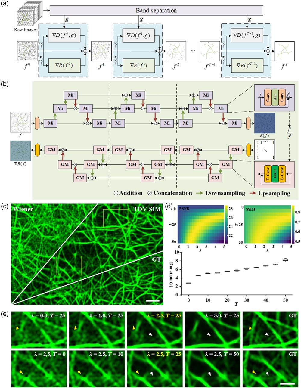
Fig. 1. TDV-SIM diagrams and parameter selection. (a) TDV-SIM reconstruction pipeline. (b) Visualization of TDV and its gradient. Mi is a residual structure micro-block and GM is its gradient. Conv is the convolution layer and T-Conv is its gradient. Act is the activation layer and GAct is its gradient. (c) Actin filaments SIM SR image. (d) Top, PSNR and SSIM of TDV-SIM reconstructions with different
![TDV-SIM outperforms other reconstruction algorithms in suppressing artifacts and hallucinations while maintaining resolution. (a) Actin filaments under the SR-SIM. (b) Magnified views of the larger boxed region in panel (a) reconstructed by Wiener deconvolution, HiFi-SIM, Hessian-SIM, and TDV-SIM. The GT image is shown as the reference. Profiles along the yellow line are on the bottom. (c) Magnified views of the smaller boxed regions in panel (a) reconstructed by Wiener deconvolution, scU-Net, DFCAN, and TDV-SIM. The GT images are shown as references. (d) Time series imaging of ER under the SR-SIM (Video 1, MP4, 45 MB [URL: https://doi.org/10.1117/1.APN.2.1.016012.s1]). (e) Magnified views of the boxed regions in panel (d) reconstructed by Wiener deconvolution, HiFi-SIM, Hessian-SIM, scU-Net, DFCAN, and TDV-SIM. The GT images are shown as references. Artifact variances of actin filaments (f) or ER tubules (g) from background regions in different reconstructions (n=15 from three cells for each sample). Yellow arrowheads in panels (c) and (e) indicate the inaccurate reconstructions of pure DL-based methods. Red arrowheads in panel (e) highlight the artifacts of physical-model-based methods. SSIM of actin filaments (h) and ER tubules (i) in different reconstructions (n=150 and 15, respectively). (j) Resolutions of different reconstructions of actin filaments in panels (a)–(c) (n=14 from three cells). Scale bars: (a) and (d) 1 μm; (b) top, (c) and (e) 0.5 μm. (b) Bottom, axial: 0.2 arbitrary units (a.u.); lateral: 0.1 μm. Data are shown as mean ± SEM. p<0.05*, p<0.01**, p<0.001***, ns: not significant (one-way ANOVA).](/richHtml/APN/2023/2/1/016012/img_002.png)
Fig. 2. TDV-SIM outperforms other reconstruction algorithms in suppressing artifacts and hallucinations while maintaining resolution. (a) Actin filaments under the SR-SIM. (b) Magnified views of the larger boxed region in panel (a) reconstructed by Wiener deconvolution, HiFi-SIM, Hessian-SIM, and TDV-SIM. The GT image is shown as the reference. Profiles along the yellow line are on the bottom. (c) Magnified views of the smaller boxed regions in panel (a) reconstructed by Wiener deconvolution, scU-Net, DFCAN, and TDV-SIM. The GT images are shown as references. (d) Time series imaging of ER under the SR-SIM (Video 1 , MP4, 45 MB [URL: https://doi.org/10.1117/1.APN.2.1.016012.s1 ]). (e) Magnified views of the boxed regions in panel (d) reconstructed by Wiener deconvolution, HiFi-SIM, Hessian-SIM, scU-Net, DFCAN, and TDV-SIM. The GT images are shown as references. Artifact variances of actin filaments (f) or ER tubules (g) from background regions in different reconstructions (
Fig. 3. TDV-SIM enables accurate reconstruction of intricate and dynamic mitochondrial cristae structures in live cells after prolonged bleaching. (a) Mitochondria under the SR-SIM. (b) Time-dependent bleaching in fluorescence intensities of mitochondria. (c) Magnified views of the larger boxed region in panel (a) reconstructed by scU-Net, DFCAN, and TDV-SIM and the corresponding GT image at 0 s. Profiles along the blue line are on the right. (d) Magnified views of the smaller boxed region in panel (a) reconstructed by Wiener deconvolution, HiFi-SIM, Hessian-SIM, and TDV-SIM and the corresponding GT images at 0, 15, and 20 s. (e) The SSIMs of regions enclosed mitochondria from different reconstructions compared to GT images at 0, 15, and 20 s (
Fig. 4. TDV-SIM enables better reconstruction of actin filaments under NL-SIM. (a) Actin filaments under the NL-SIM. (b), (c) Magnified views of the white boxed regions in panel (a) reconstructed by Wiener deconvolution, Hessian-SIM, DFCAN, and TDV-NL-SIM. The GT image is shown as the reference. Profiles along the yellow line are on the bottom. (d) Magnified views of the yellow boxed regions in panel (a) reconstructed by Wiener deconvolution, Hessian-SIM, DFCAN, and TDV-NL-SIM. The GT image is shown as the reference. Yellow arrowheads indicate the inaccurate reconstructions of pure DL-based methods. (e) Artifact variances of actin filaments from background regions in different reconstructions (

Set citation alerts for the article
Please enter your email address
© Copyright 2018-2021 | Chinese Laser Press. All Rights Reserved 沪ICP备15018463号-20