
Zebin Su, Min Gao, Pengfei Li, Junfeng Jing, Huanhuan Zhang. Digital Printing Defect Classification Algorithm Based on Convolutional Neural Network[J]. Laser & Optoelectronics Progress, 2020, 57(24): 241011
- Laser & Optoelectronics Progress
- Vol. 57, Issue 24, 241011 (2020)
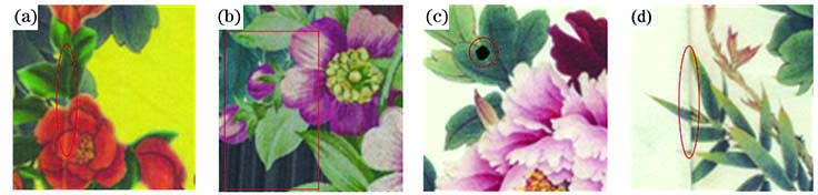
Fig. 1. Examples of digital printing defects. (a) PASS tracks; (b) uneven inkjet; (c) ink leakage; (d) fabric wrinkles
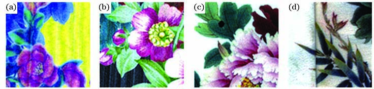
Fig. 2. RGB color space histogram equalization processing results. (a) PASS tracks; (b) uneven inkjet; (c) ink leakage; (d) fabric wrinkles
Fig. 3. Gaussian filtering processing results. (a) PASS tracks; (b) uneven inkjet; (c) ink leakage; (d) fabric wrinkles
Fig. 4. Adjustment results of image resolution based on local mean algorithm. (a) Before resolution adjustment; (b) after resolution adjustment
Fig. 5. Image data enhancement results. (a) Original image; (b) flip vertically; (c) horizontal mirroring; (d) rotate 90°; (e) rotate 180°; (f) rotate 270°
Fig. 6. Flow chart of classification algorithm
Fig. 7. Topological structure of convolutional neural network
Fig. 8. Samples of digital printing defect data set. (a)--(d) PASS tracks; (e)--(h) uneven inkjet; (i)--(l) ink leakage; (m)--(p) fabric wrinkles
Fig. 9. Total loss rate curve
Fig. 10. Kappa coefficient value predicted by different CNN models
|
Table 1. Comparison of defect features in digital printing
|
Table 2. Classification accuracy corresponding to different objective functions
|
Table 3. Classification accuracy corresponding to different optimization algorithms
| |||||||||||||||||||||||||||||||||||||||||||||||||||||||||||||||||||||||||||||||||||||||||||
Table 4. Performance index of each defect classification
|
Table 5. Training and testing time of different CNN models

Set citation alerts for the article
Please enter your email address
© Copyright 2018-2021 | Chinese Laser Press. All Rights Reserved 沪ICP备15018463号-20