Author Affiliations
1State Key Laboratory of Advanced Optical Communication Systems and Networks, School of Physics and Astronomy, Shanghai Jiao Tong University, Shanghai 200240, China2Interdisciplinary Center for Quantum Information and State Key Laboratory of Modern Optical Instrumentation, Zhejiang Province Key Laboratory of Quantum Technology and Device, and School of Physics, Zhejiang University, Hangzhou 310027, China3MOE Key Laboratory of Advanced Micro-Structured Materials, School of Physics Science and Engineering, Tongji University, Shanghai 200092, China4Shanghai Research Center for Quantum Sciences, Shanghai 201315, China5Collaborative Innovation Center of Light Manipulations and Applications, Shandong Normal University, Jinan 250358, China6e-mail: yuanluqi@sjtu.edu.cn7e-mail: yang_yaping@tongji.edu.cn8e-mail: xfchen@sjtu.edu.cnshow less
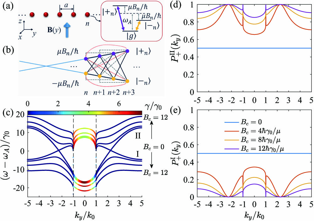
Fig. 1. (a) Schematic of a 1D V-type atomic array under a magnetic field B(y). (b) Schematic of the corresponding lattice where the nth atom has non-degenerate excited states |±n⟩ with frequency shifted by ±μBn/ℏ. Blue lines indicate a linear trend of Bn as in Eq. (2). (c) Band structures with different constant magnetic fields Bc with values Bc=0,4ℏγ0/μ,8ℏγ0/μ,12ℏγ0/μ, respectively. Black arrows indicate values of Bc for corresponding bands. Decay rates of modes are color coded. Probabilities of eigenstates on (d) band II and (e) band I projected on |+⟩ states for different Bc. Here, a=0.1λ.
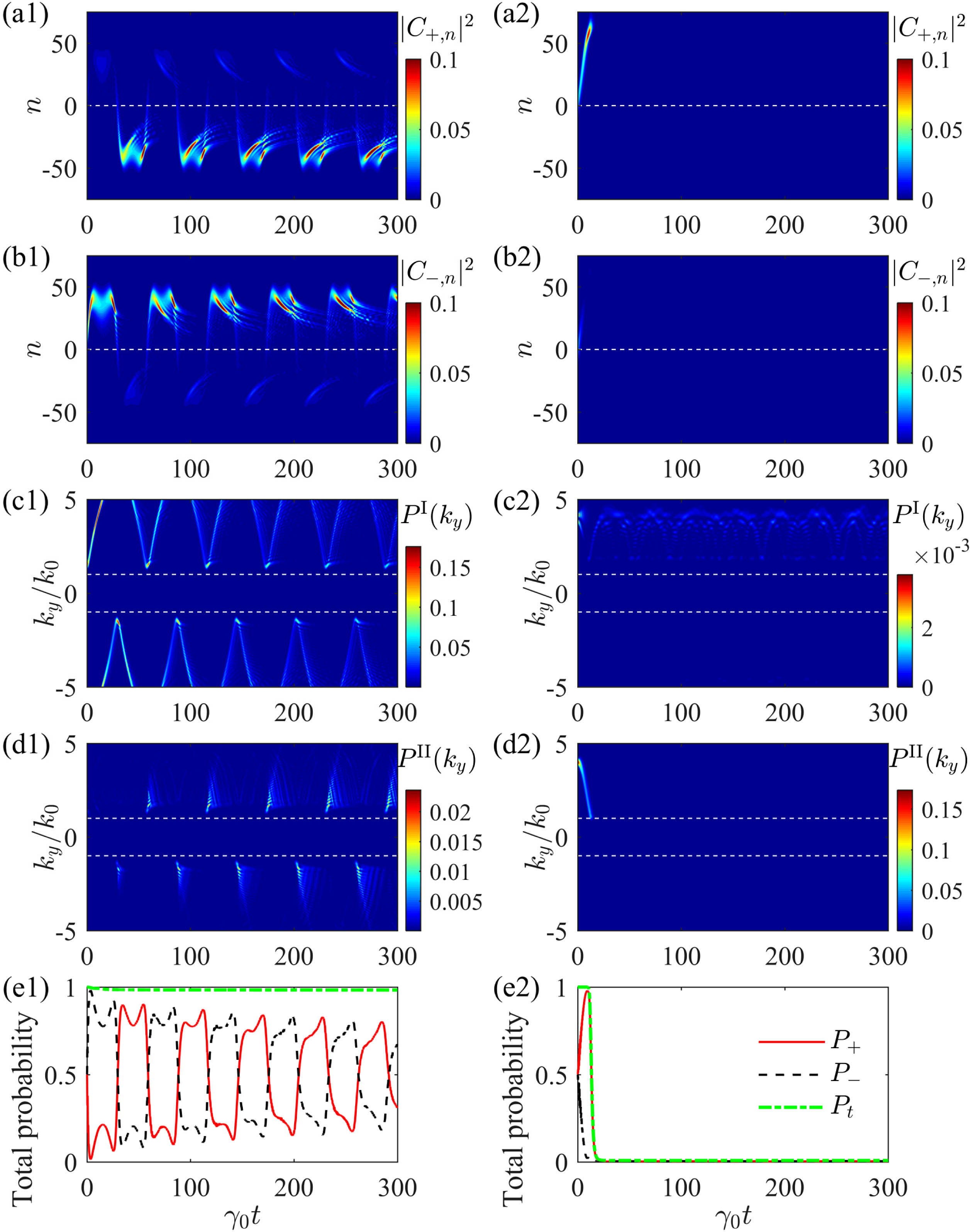
Fig. 2. Bloch oscillations for Gaussian excitations initially centered at nc=0 with kc=1.5k0 on band I (left) and kc=4k0 on band II (right), shown by temporal evolution for excitation probabilities of (a1), (a2) |C+,n|2; (b1), (b2) |C−,n|2; (c1), (c2) PI(ky); (d1), (d2) PII(ky); (e1), (e2) P+, P−, and Pt. Here, a=0.1λ and μB0/ℏ=0.2γ0.
Fig. 3. Bloch oscillations for Gaussian excitations initially centered at nc=0 and kc=k0 on band I with a static magnetic field (left) and a controllable magnetic field (right), whose zero point is shifted to y=30a over a time period from 0 to 20γ0−1 and back to y=0 over a time period from 180γ0−1 to 200γ0−1, shown by temporal evolution of (a1), (a2) Pn; (b1), (b2) PI+PII; (c1), (c2) P+, P−, and Pt. Other parameters are the same as those in Fig. 2.
Fig. 4. Bloch oscillations for a Gaussian excitation initially centered at nc=0 with kc=1.5k0 (left) and kc=3k0 (right) on band I. Temporal evolution of (a1), (a2) Pn=|C+,n|2+|C−,n|2 and (b1), (b2) PI(ky)+PII(ky) in an array with atomic number N=201 within a time period of 300 γ0−1 after t=108 γ0−1 (left) and after t=1013 γ0−1 (right). (c1), (c2) The total probability Pt versus order of magnitude of time for N=51 (blue solid line), N=101 (green dash-dotted line), N=151 (red dash line), and N=201 (black dotted line). a=0.1λ and μB0/ℏ=0.2γ0.
Fig. 5. Bloch oscillations started from nc=0 for Gaussian excitations initially centered at kc=4k0 on band I (left), kc=2k0 on band II (middle), and kc=−0.5k0 on band II (right), shown by temporal evolutions of (a1)–(a3) Pn, (b1)–(b3) PI(ky)+PII(ky), (c1), (c2) total excitation probabilities P+ (red solid line), P− (black dash line), and Pt (green dash-dotted line). An exponential function is used to fit the decay of the total excitation probability in (c3) (blue dotted line). Here, N=201, a=0.1λ, and μB0/ℏ=0.2γ0.
Fig. 6. Bloch oscillations started from nc=50 for a Gaussian excitation initially centered at kc=1.5k0 on band I, shown by the temporal evolution of (a) Pn, (b) PI+PII, (c) P+ (red solid line), P− (black dash line), and Pt (green dash-dotted line). Here N=201, a=0.1λ, and μB0/ℏ=0.2γ0.
Fig. 7. Numerically calculated decay rates in descending order of single-excitation eigenstates in an atomic array under a linear magnetic field with varying μB0/ℏγ0 indicated by different colors for (a) a=0.1λ, N=201; (b) a=0.1λ, N=101; and (c) a=0.2λ, N=201.
Fig. 8. Decay rates of the most subradiant single-excitation modes with (a) increasing spatial disorder characterized by the deviation width δa and (b) increasing Doppler broadening ΔD for B0=0 (blue dash line) and B0=0.2ℏγ0/μ (red solid line). a=0.1λ and N=201.