The z-scan technique, after being introduced by Sheik-Bahae et al. in 1989^[1,2], has been widely adopted for characterizing nonlinear optical coefficients of optical materials. Theoretical curves calculated by the model can fit experimental data elegantly for z-scan experiments with continuous-wave lasers^[3,4]. However, in many reports adopting pulsed lasers, especially with femtosecond (fs) pulse width, poor fitting has been quite commonly encountered with the accompanying large deviation between theoretical curves and experimental data, both for open-aperture (OA) transmittance^[5–7] and closed-aperture (CA) transmittance^[8–11]. Furthermore, there is a lack of consistency between the nonlinear parameters extracted from the same substance in different reports. For example, the extracted results of carbon disulfide (CS2) may span over 10−18−10−20m2/W for the third-order nonlinear refraction (NLR) coefficient (γ) and 10−13-10−16m/W for the third-order nonlinear absorption (NLA) coefficient (β), respectively^[8,12–26]. Such a large discrepancy of extracted parameters and the phenomenon of poor fitting cannot be simply attributed to experimental errors, but needs theoretical re-examination.

Sheik-Bahae’s model (SBM)^[1,2] adopts the thin sample approximation, based on which the intensity distribution in a plane behind the sample is analytically calculated using the classical nonlinear differential equation (NLDE)^[27–29]. It has been pointed out that the effect of optical NLR or NLA is influenced by the nonlinear optical coefficient and the sample thickness, as well as the laser intensity^[1,2,8]. Obviously, sample thickness is not the only factor affecting accuracy, but the comprehensive effect of experimental conditions. The extracted nonlinear optical coefficients show dependence on laser intensity^[8], which is against common understanding of physics. Efforts have been made to explore new theoretical approaches, such as the Huygens–Fresnel principle^[30], Gaussian beam characteristic parameter transformation^[31], classical NLDE combined with Gaussian decomposition based on temporal differential^[32], and modified NLDE by nonlocal principle combined with Gaussian decomposition^[33,34]. The aspect of numerical calculation has been investigated as well, such as FFT^[35] and classical NLDE combined with the Fresnel–Kirchhoff diffraction principle^[36]. The curve fitting of CA transmittance data can be improved for the case with large NLR by the use of the Fresnel–Kirchhoff diffraction principle for calculating the CA electric field^[30,36], but there is currently no effective measure to improve the curve fitting of OA transmittance data. Note that the adoption of NLDE^[32–34] is still based on the thin sample approximation^[1,2], and thus it is difficult to make radical improvements. Theoretical models adequate for a thick sample with strong nonlinearity have been investigated. The nonlinear paraxial wave equation (NPWE) in expression of NLR and NLA coefficients was solved and followed by the Huygens–Fresnel principle^[37], and the nonlinear Schrödinger equation was solved using a finite difference beam propagation approach^[38]. A generic approach for z-scan calculation has to be based on solving the wave equation for a nonlinear medium. Nevertheless, the existing issue of inconsistent nonlinear coefficients extracted from theoretical fitting with z-scan experimental data in different experimental conditions has yet to be addressed, which is essential for the application of the nonlinear characteristics of materials^[39,40].

In this Letter, we investigate the consistency of nonlinear optical coefficients extracted from z-scan measurements with different sample thicknesses and laser intensities. To solve the wave equation, the propagation of Gaussian beam in the nonlinear medium^[41] is utilized, and the Fresnel–Kirchhoff diffraction integral is applied to further obtain the intensity distribution in the aperture plane. The experimental data of CS2 are fitted by this beam propagation diffraction model (BPDM) for samples with different thicknesses at different laser intensities. We show that nonlinear optical coefficients extracted by BPDM maintain constancy regardless of sample thickness and laser intensity, through which experimentalists can verify the reliability of their obtained results.

In the z-scan configuration, the sample of a thickness L is placed at a position z, with z=0 for the waist position of the incident Gaussian beam. The electric field of a propagating beam inside the sample is expressed using a coordinate system (r,zb) as in slowly varying envelope approximation. Using Eq. (1), the wave equation can be rewritten as where D^=−iΔt/2k and S^=−(ik/2n02)(1−n02+χ). Here, Δt is the transverse Laplacian, n0 is the real part of the linear refractive index, and k is the wave vector. The electric susceptibility χ only retains terms up to the third order, i.e., χ=χ(1)+χ(3)|U(r,zb)|2, but may be extended to incorporate higher-order terms for generic cases. D^ accounts for the diffraction effect by the linear beam propagation in the medium, and S^ accounts for the nonlinear absorption effect and the NLR effect. The SBM takes the thin sample approximation such that the beam diffraction during propagation in the sample is ignored. In contrast, with beam propagation, Eq. (2) takes into account the diffraction due to inhomogeneity of the medium, which is caused by the NLR resulting from the electric field distribution throughout the sample, thus eliminating the need for the thin sample approximation.

The numerical solution of Eq. (2) starts from the entrance plane of the sample, i.e., U(r,zb=0), to the exit plane, i.e., U(r,zb=L), iteratively. Upon exiting the sample, the electric field is expressed as

After emerging from the sample, the beam reaches the aperture plane via Fraunhofer diffraction. The electric field at the aperture plane can be calculated by the Fresnel–Kirchhoff diffraction integral: where d is the distance between the exit plane of the sample and the aperture plane for signal detection. The normalized transmittance can be obtained by spatially integrating Ea(ρ) in the aperture for the CA measurement and by spatially integrating Ee(r) in the exit plane of the sample for the OA measurement. Here, we co-fit OA and CA experimental data to obtain two nonlinear coefficients simultaneously by joining numerical calculation with the genetic algorithm.

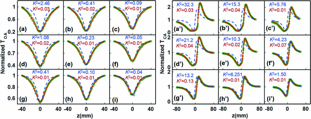
A 50 fs pulsed laser at a wavelength of 800 nm with a pulse repetition frequency of 1 kHz was adopted in the z-scan experiment. Samples were CS2 contained in cuvettes with inner gaps of 0.5 mm, 1 mm, and 2 mm and were tested at peak intensities of 967GW/cm2, 764GW/cm2, and 500GW/cm2. Figure 1 shows the measured OA and CA transmittances by scanning the sample position at z. The normalized transmittances in OA and CA cases can be nicely fitted. The curve fittings shown in Fig. 1 visually demonstrate that BPDM has excellent performance for all sample cases. Chi-square goodness of fit test K2 was defined as K2=∑(Mj−Cj)2/Cj, where Mj and Cj are the jth normalized transmittance data obtained by z-scan measurements or numerical calculation by the use of the theoretical model of the z-scan technique, respectively. For clarity, the magnitudes of chi-square goodness of fit test K2 are shown in Fig. 1 as the quantitative measure to their curve-fitting performances.

Since NLR is ignored in the SBM fitting of OA transmittance data when solving the NLA coefficient, the intensity profiles maintain the Gaussian curve shape. However, as revealed by BPDM in Fig. 2(c), the intensity distribution profile strongly deviates from the Gaussian distribution due to the diffraction effect of strong NLR at the position of the laser waist, i.e., z=0mm. In practice, the SBM fitting is usually forced to match the experimental data at z=0mm and the both ends simultaneously. Thus, while achieving the best agreement with the non-Gaussian intensity profile at z=0mm [Fig. 2(c)], NLA is apparently underestimated, giving a higher intensity distribution profile [Figs. 2(b) and 2(d)] and higher OA transmittance [Fig. 2(a)] in regions between z=0mm and the two ends, e.g., at z=−25,20mm. Also, fitting the numerically calculated field to a Gaussian distribution^[35] is inadequate in such a situation.

The different phase distribution profiles calculated by two models shown in Figs. 2(b’)–2(d’) can explain the differences in the CA transmittances. At z=0mm, the phase lag obtained obviously deviates from the Gaussian curve shape. Hence, the assumption of Gaussian distributions of intensity and phase shift in SBM deviates from the real situation and makes it hard to fit skewed CA transmittance curves, i.e., with a narrow peak and wide valley herein, which had also been observed in previous reports^[32,42]. The Fresnel–Kirchhoff diffraction principle should be applied to calculate the electric field distribution at the far-field aperture plane instead, as the Gaussian decomposition method does not have good performance on non-Gaussian beams.

By plotting the extracted nonlinear optical coefficients γ and β versus the product of the incident light intensity and the sample thickness I0·L as shown in Fig. 3, we see that BPDM provides constant results to I0·L, i.e., β=5.0×10−13m/W and γ=2.0×10−19m2/W, denoting that the contribution of the fifth-order nonlinearity or other higher-order nonlinearity is negligible within the experimental range of laser intensity. By taking the aforementioned γ and β values, the lines of q0=1 and ΔΦ0=1 are denoted in Fig. 3 for q0=βI0L and ΔΦ0=kγI0L. It is seen that the results of these two models are close for q0<1 and ΔΦ0<1, as the limiting condition for applying SBM^[1,2]. However, practically, it is hard to comply with this condition without knowing the values of β and γ beforehand. A series of experimental results taken from references are denoted in Fig. 3, and it is seen that some fall out of such a regime. In contrast, BPDM sets z-scan experiments free from this limiting condition. Moreover, the 95% confidence interval becomes broad with decreasing I0·L, because experimentally the signal-to-noise ratio becomes poor upon a reduced nonlinear optical signal. This trend is also illustrated by the reported results. By applying BPDM, the experiment can be done at high levels of I0·L to acquire more accurate results. Also, the constancy of extracted nonlinear optical coefficients via varying incident light intensity or sample thickness can be used to confirm whether a z-scan experiment is properly conducted, which is exactly the significance of discussing the sample thickness and light intensity^[43,44].

In conclusion, the issue of inconsistent nonlinear optical coefficients extracted from z-scan measurements with different sample thicknesses and different laser intensities has been addressed. The BPDM is developed to solve the wave equation based on the propagation of the Gaussian beam in a nonlinear medium and obtain the far-field intensity distribution in the aperture plane based on the Fresnel–Kirchhoff diffraction integral principle. NLR, NLA, and diffraction for beam propagation within a sample will all have an effect on the electric field redistribution with propagation, including intensity and phase, which have been taken into account. Hence, thin sample approximation is eliminated, and the laser intensity need not be deliberately limited to trade off experimental accuracy. The determined third-order nonlinear parameters of CS2 (β=5.0×10−13m/W and γ=2.0×10−19m2/W) maintain constancy regardless of sample thickness and laser intensity, which not only clarifies the physical significance of optical parameters but also reveals negligible contributions of the fifth-order nonlinearity within the experimental range of laser intensity. The constancy of extracted parameters to the incident light intensity can be taken as a measure to check the goodness of the z-scan measurement.

References

[1] M. Sheik-Bahae, A. A. Said, E. W. Van Stryland. Opt. Lett., 14, 955(1989).
[2] M. Sheik-Bahae, A. A. Said, T.-H. Wei, D. J. Hagan, E. W. Van Stryland. IEEE J. Quantum Electron., 26, 760(1990).
[3] K. K. Nagaraja, S. Pramodini, P. Poornesh, M. P. Telenkov, I. V. Kityk. Physica B, 512, 45(2017).
[4] N. A. Zulina, M. A. Baranov, K. I. Kniazev, V. O. Kaliabin, I. Y. Denisyuk, S. U. Achor, V. E. Sitnikova. Opt. Laser Technol., 103, 396(2018).
[5] M. B. M. Krishna, N. Venkatramaiah, R. Venkatesan, D. N. Rao. J. Mater. Chem., 22, 3059(2012).
[6] K. P. Wang, J. Wang, J. T. Fan, M. Lotya, A. O’Neill, D. Fox, Y. Y. Feng, X. Y. Zhang, B. X. Jiang, Q. Z. Zhao, H. Z. Zhang, J. N. Coleman, L. Zhang, W. J. Blau. ACS Nano, 7, 9260(2013).
[7] R. A. Ganeev, M. Baba, A. I. Ryasnyansky, M. Suzuki, H. Kuroda. Opt. Commun., 240, 437(2004).
[8] R. A. Ganeev, A. I. Ryasnyansky, M. Baba, M. Suzuki, N. Ishizawa, M. Turu, S. Sakakibara, H. Kuroda. Appl. Phys. B, 78, 433(2004).
[9] S. Lu, C. Zhao, Y. Zou, S. Chen, Y. Chen, Y. Li, H. Zhang, S. Wen, D. Tang. Opt. Express, 21, 2072(2013).
[10] X. L. Zhang, Z. B. Liu, X. C. Li, Q. Ma, X. D. Chen, J. G. Tian, Y. F. Xu, Y. S. Chen. Opt. Express, 21, 7511(2013).
[11] B. Can-Uc, R. Rangel-Rojo, A. Peña-Ramírez, C. B. de Araújo, H. T. M. C. M. Baltar, A. Crespo-Sosa, M. L. Garcia-Betancourt, A. Oliver. Opt. Express, 24, 9955(2016).
[12] M. Falconieri, G. Salvetti. Appl. Phys. B, 69, 133(1999).
[13] S. Couris, M. Renard, O. Faucher, B. Lavorel, R. Chaux, E. Koudoumas, X. Michaut. Chem. Phys. Lett., 369, 318(2003).
[14] A. Gnoli, L. Razzari, M. Righini. Opt. Express, 13, 7976(2005).
[15] T. Kawazoe, H. Kawaguchi, J. Inoue, O. Haba, M. Ueda. Opt. Commun., 160, 125(1999).
[16] H. S. Albrecht, P. Heist, J. Kleinschmidt, D. V. Lap. Appl. Phys. B: Photophys. Laser Chem., 57, 193(1993).
[17] S. Couris, E. Koudoumas, F. Dong, S. Leach. J. Phys. B: Atom. Mol. Opt. Phys., 29, 5033(1996).
[18] M. Reichert, H. Hu, M. R. Ferdinandus, M. Seidel, P. Zhao, T. R. Ensley, D. Peceli, J. M. Reed, D. A. Fishman, S. Webster, D. J. Hagan, E. W. Van Stryland. Optica, 1, 436(2014).
[19] G. Boudebs, K. Fedus. J. Appl. Phys., 105, 103106(2009).
[20] D. G. Kong, Q. Chang, H. Ye, Y. C. Gao, Y. X. Wang, X. R. Zhang, K. Yang, W. Z. Wu, Y. L. Song. J. Phys. B: Atom. Mol. Opt. Phys., 42, 065401(2009).
[21] R. A. Ganeev, A. I. Ryasnyansky, N. Ishizawa, M. Baba, M. Suzuki, M. Turu, S. Sakakibara, H. Kuroda. Opt. Commun., 231, 431(2004).
[22] X. Liu, S. Guo, H. Wang, N. Ming, L. Hou. J. Nonlinear Opt. Phys. Mater., 10, 431(2001).
[23] I. P. Nikolakakos, A. Major, J. S. Aitchison, P. W. E. Smith. IEEE J. Sel. Top. Quantum Electron., 10, 1164(2004).
[24] K. Minoshima, M. Taiji, T. Kobayashi. Opt. Lett., 16, 1683(1991).
[25] D. I. Kovsh, S. Yang, D. J. Hagan, E. W. Van Stryland. Appl. Opt., 38, 5168(1999).
[26] X. Q. Yan, Z. B. Liu, S. Shi, W. Y. Zhou, J. G. Tian. Opt. Express, 18, 26169(2010).
[27] S. Chen, S. Yang, Y. Huang, W. Jiao, G. Fan, Y. Gao. Chin. Opt. Lett., 18, 011901(2020).
[28] Y. Han, B. Gu, S. Zhang, G. Rui, J. He, Y. Cui. Chin. Opt. Lett., 17, 061901(2019).
[29] X. Peng, Y. Zhao, Y. Wang, G. Hu, L. Yang, J. Shao. Chin. Opt. Lett., 16, 051601(2018).
[30] R. E. Samad, N. D. Vieira. J. Opt. Soc. Am. B: Opt. Phys., 15, 2742(1998).
[31] C. H. Kwak, Y. L. Lee, S. G. Kim. J. Opt. Soc. Am. B: Opt. Phys., 16, 600(1999).
[32] S. Q. Chen, Z. B. Liu, W. P. Zang, J. G. Tian, W. Y. Zhou, F. Song, C. P. Zhang. J. Opt. Soc. Am. B: Opt. Phys., 22, 1911(2005).
[33] E. V. Garcia Ramirez, M. L. Arroyo Carrasco, M. M. Mendez Otero, E. Reynoso Lara, S. Chavez-Cerda, M. D. Iturbe Castillo. J. Opt., 13, 085203(2011).
[34] A. Balbuena Ortega, M. L. Arroyo Carrasco, M. M. Méndez Otero, E. Reynoso Lara, E. V. García Ramírez, M. D. Iturbe Castillo. Opt. Express, 22, 27932(2014).
[35] S. Hughes, J. M. Burzler, G. Spruce, B. S. Wherrett. J. Opt. Soc. Am. B: Opt. Phys., 12, 1888(1995).
[36] B. Yao, L. Ren, X. Hou. J. Opt. Soc. Am. B: Opt. Phys., 20, 1290(2003).
[37] L. Pálfalvi, B. C. Tóth, G. Almási, J. A. Fülöp, J. Hebling. Appl. Phys. B: Lasers Opt., 97, 679(2009).
[38] D. Namarathne, S. Walden, M. Shortell, E. Jaatinen. Appl. Phys. A: Mater. Sci. Process., 122, 319(2016).
[39] S. Basudeb, M. Cedrik, Z. Thomas. Adv. Photon., 1, 024002(2019).
[40] R. Shimon, F. Yeshaiahu. Adv. Photon., 1, 066003(2019).
[41] K. Pieszyński. Scientific Bulletin. Physics, 29, 65(2008).
[42] E. Koushki, A. Farzaneh, S. H. Mousavi. Appl. Phys. B: Lasers Opt., 99, 565(2010).
[43] R. E. Bridges, G. L. Fischer, R. W. Boyd. Opt. Lett., 20, 1821(1995).
[44] P. Chen, D. A. Oulianov, I. V. Tomov, P. M. Rentzepis. J. Appl. Phys., 85, 7043(1999).