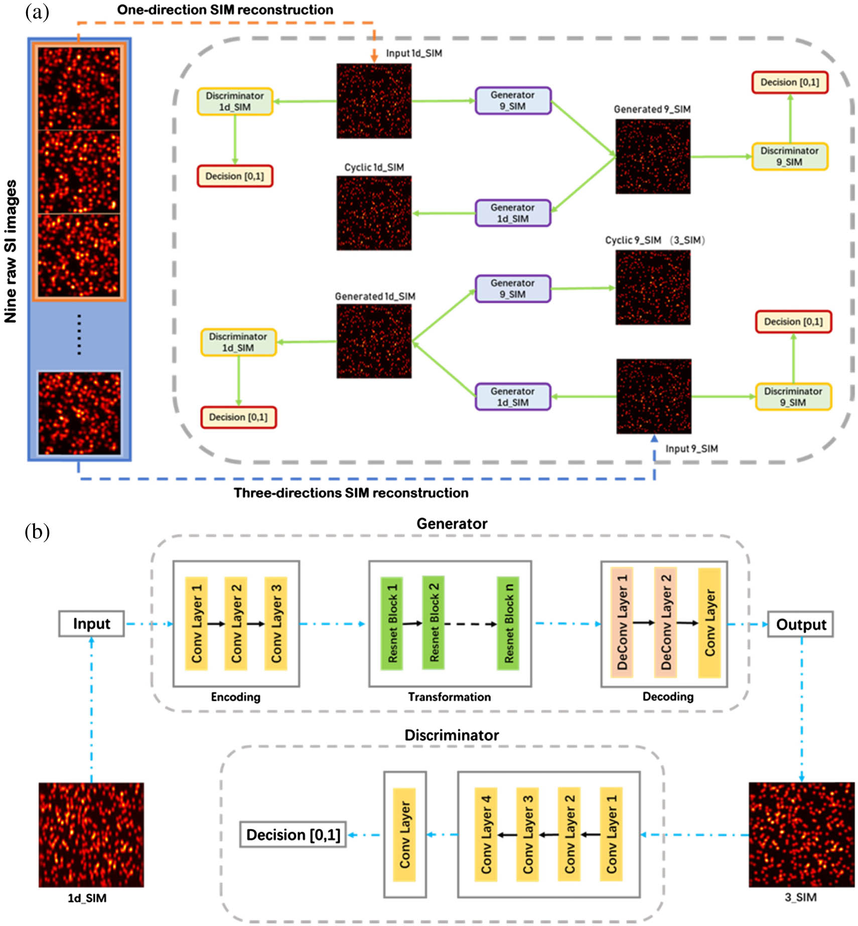
Fig. 1. Schematics of the deep neural network trained for SIM imaging. (a) The inputs are 1d_SIM and 9_SIM images generated by nine lower-resolution raw images (using the SIM algorithm) as two training datasets with different training labels. The deep neural network features two generators and two discriminators. These generators and discriminators are trained by optimizing various parameters to minimize the adversarial loss between the network’s input and output as well as cycle consistency loss between the network’s input image and the corresponding cyclic image. The cyclic 9_SIM in the schematics is the final image (3_SIM) desired. (b) Detailed schematics of half of the CycleGAN training phase (generator 1d_SIM and discriminator 9_SIM). The generator consists of three parts: an encoder (which uses convolution layers to extract features from the input image), a converter (which uses residual blocks to combine different similar features of the image), and a decoder (which uses the deconvolution layer to restore the low-level features from the feature vector), realizing the functions of encoding, transformation, and decoding. The discriminator uses a 1D convolution layer to determine whether these features belong to that particular category. The other half of the CycleGAN training phase (generator 9_SIM and discriminator 1d_SIM) is the same as this.

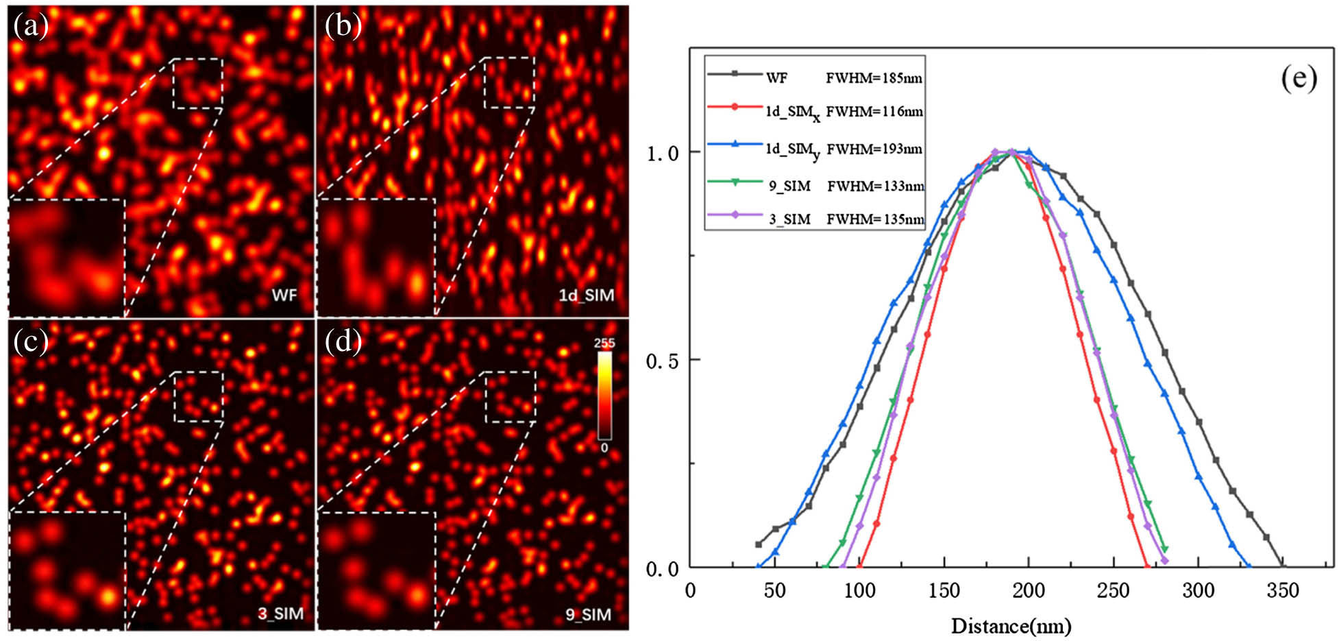
Fig. 2. Experimental comparison of imaging modes with a database of point images. For all methods, nine raw SI images were used as the basis for processing. (a) The WF image was generated by summing all raw SI images. (b) 1d_SIM images were generated by three raw SI images in the x direction. (c) The 3_SIM images formed the output of the CNN training. (d) 9_SIM image reconstructed from nine SI raw images as the ground truth. The enlarged area shows neighboring beads in the dashed box. In both the 3_SIM and the 9_SIM images, the beads are distinguishable and yield a resolution beyond the diffraction limit, which 1d_SIM images cannot realize. The resolution of the point is shown in (e).

Fig. 3. Using deep learning to transform images in the dataset of lines from 1d_SIM to 9_SIM. (a) WF line image. (b) 1d_SIM line image used as network input. (c) 3_SIM line image used as network output. (d) 9_SIM line image used as contrast. (e) The achieved resolution of different approaches of line images.

Fig. 4. Deep learning-enabled transformation of images of curves from 1d_SIM to 9_SIM. (a) WF curve image. (b) 1d_SIM image of curves used as input to the neural network. (c) 3_SIM image that was the network output, compared to the (d) 9_SIM image.

Fig. 5. Experimental setup for the TIRF-SIM. A laser beam with a wavelength of 532 nm was employed as the light source. After expansion, the light was illuminated into digital micromirror device (DMD) and generated structured illumination. A polarizer and a half-wave plate were used to rotate the polarization orientation; a spatial mask is used to filter the excess frequency components. The generated structured illumination is tightly focused by a high-numerical-aperture (NA) oil-immersion objective lens (Olympus, NA=1.4, 100×) from the bottom side onto the sample. The sample was fixed at a scanning stage and was prepared with the following procedures. A droplet of dilute nanoparticles (100 nm, attached with R6G molecules) suspension was subsequently dropped onto the prepared cover slip and evaporated naturally. After rinsing with water and air drying, the sample was ready for use.

Fig. 6. Comparison of the experiment results of deep learning [(c) 3_SIM]) with (a) WF, (b) 1_direction SIM, and (d) 9_SIM. Wide-field images were generated by summing all raw images, 1d_SIM images were reconstructed using three SI raw images in one direction (x), and the 9_SIM images were reconstructed from all nine SI raw images and used as ground truth compared with the 3_SIM images. The 1d_SIM image was used as input to the network to generate the 3_SIM images. The dotted frame in the figures shows an enlarged view of two areas (A and B), where the intensity distribution of the white dotted line is shown in the line chart on the right. In (a), two closely spaced nanobeads that could not be resolved by TIRF microscopy, and the 1d_SIM image super-resolved in one direction in (b). The trained neural network took the 1d_SIM image as input and resolved the beads, agreeing well with the SIM images.

Fig. 7. Fourier analysis of the reconstructed images. (a) Comparison of the frequency spectrum of images with different numbers of Gaussian points. The frequency spectrum of the Gaussian points is highly symmetrical. (b) The different colors indicate different types of frequency-related information. The yellow area represents the frequency-related information of the original image, and the green area represents information restored by the network. The grid in (b) represents the relationship between the available frequency-related information and the frequency-related information recovered by the network. (c) The Fourier transform of the reconstructions in Fig. 2 was used to obtain the spectra. To illustrate the Fourier coverage of each model, three circles are marked in each image, where the green–yellow circle corresponds to support for the WF image, the blue circle corresponds to that for the 1d_SIM image, and the yellow circle represents support for the 3_SIM and 9_SIM images.

Fig. 8. Comparing WF to 9_SIM with 1d_SIM to 9_SIM. (a) The 9_SIM image reconstructed from nine SI raw images. (b)–(d) Network output, 200, 500, and 900 image pairs (1d_SIM and 9_SIM) were used to train the network models, respectively. (e)–(h) Network output, using 100, 200, 500, and 900 image pairs (WF and 9_SIM) as datasets to train the network models. Each network underwent 10,000 iterations. Some details were not correctly restored in the WF-to-9_SIM training model. The arrows in (a)–(h) point to a missing detail.

Table 1. Performance Metrics of the Proposed Method on the Testing Data