Abstract
This study shows that convolutional neural networks (CNNs) can be used to improve the performance of structured illumination microscopy to enable it to reconstruct a super-resolution image using three instead of nine raw frames, which is the standard number of frames required to this end. Owing to the isotropy of the fluorescence group, the correlation between the high-frequency information in each direction of the spectrum is obtained by training the CNNs. A high-precision super-resolution image can thus be reconstructed using accurate data from three image frames in one direction. This allows for gentler super-resolution imaging at higher speeds and weakens phototoxicity in the imaging process.1. INTRODUCTION
Fluorescence microscopy is an important tool in the life sciences for observing cells, tissues, and organisms. However, the Abbe diffraction limit [1] implies that the spatial resolution of the fluorescence microscope can attain only half the wavelength of incident light. Recently developed techniques in microscopy, such as stochastic optical reconstruction microscopy (STORM) [2,3], photoactivated localization microscopy (PALM) [4,5], structured illumination microscopy (SIM) [6,7], stimulated emission depletion (STED) [8,9], and other super-resolution microscopy [10–12] can help overcome this limit to enable the imaging of biological processes in cells at higher resolution.
Owing to its low phototoxicity and high frame rate acquisition, SIM stands out among these techniques to achieve optical super-resolution in bio-imaging [13]. In general, SIM enhances resolution by encoding high spatial frequencies of the sample in structured patterns (typically sinusoidal to affect the formation of the Moiré pattern). By measuring the frequency of the Moiré pattern in the observed image and the known frequency of the pattern of illumination, the unknown frequency content of the specimen can be computed. In linear SIM, it is theoretically up to twice the frequency limit, which is imposed by the optical transfer function (OTF) of the optical system. In nonlinear SIM [14], by the use of the nonlinear effect of fluorescence, it could reach more times the frequency limit.
To compute unknown frequencies from raw data, SIM requires three images with shifting illumination patterns to separate mixed spatial frequencies along a given orientation. To enhance isotropic resolution, this process is performed three times with illumination patterns obtained at different angles and requires a total of nine raw images per super-resolved (SR) SIM image, which means that the sample needs to be repeatedly exposed. Thus, reducing number of raw images in SIM reconstruction has been researched in recent years. SR image reconstruction using three [15–17] and four [18] raw frames of structured illumination (SI) has been implemented to increase the speed of acquisition of the images and reduce phototoxic effects. But these methods require assumptions about the process of formation of the image, and the final results are limited by the imaging environment and type of noise. For example, in the deconvolution method [19], this requires a precise understanding of the optics and well-characterized noise-related statistics. This has led to the design of such popular algorithms as the joint Richardson–Lucy deconvolution [18,20], which requires knowledge of the point-spread function of the microscope and assumes Poisson noise statistics to estimate missing information in SIM. However, such algorithms are limited by the accuracy of their assumptions and thus cannot capture the full statistical complexity of microscopic images.
Sign up for Photonics Research TOC. Get the latest issue of Photonics Research delivered right to you!Sign up now
Machine learning [21] has been used more commonly in recent years with advances in computational performance. The core concept of machine learning is to find a rule to realize a correlation between the input and the output. This process is carried out using a large amount of tagged data. Deep learning (DL) [22] is a method of machine learning in which the “deep” refers to the depth of the model, which emphasizes learning from successive layers and looking for increasingly meaningful representations.
The DL framework does not explicitly use any model or prior knowledge, and instead relies on large datasets to “learn” the underlying inverse problem. The convolutional neural networks (CNNs) [23] are in a category of deep learning that can obtain excellent results in problems of image processing and computer vision tasks. Its outcome has two important components. First, the result of the training stage is a CNN that corresponds to a plausible underlying mapping function relating the measurement to the solution. Second, the trained CNN can be used to make “predictions” when presented with new measurements that were not used in the training stage.
In recent years, deep learning methods have been applied to super-resolution microscopic imaging, such as the regular optical microscopes [24], PALM [25], STORM [26], and Fourier ptychographic microscopy [27], and they have achieved good results.
The paper proposes the use of a deep-learning-based framework to reconstruct SIM images using fewer frames than are currently required. The cycle-consistent generative adversarial network (CycleGAN) is used to reconstruct the super-resolution image (we called it 3_SIM) through the single-direction phase shift of three raw SI images (we called them 1d_SIM). Owing to the characteristics of the CycleGAN, the data in train A and train B do not need to correspond one to one. The network can be trained without using paired training data, which reduces the number of training steps needed and saves time. Our method does not require assumptions about the modeling of the process of image formation, and instead creates a super-resolved image directly from the raw data. It requires only three SI images in a given direction and reconstructs a 1d_SIM image, and it can generate a 3_SIM image with a reconstruction resolution comparable to the traditional linear SIM methods. This method is parameter free, requires no expertise on the part of the user, is easy to implement on any SIM dataset, and does not rely on prior knowledge of the structure in the sample.
2. Methods
A. Cycle-Consistent Generative Adversarial Networks
Generative adversarial networks (GANs) [28] constitute an approach to deep learning proposed by Ian Goodfellow in 2014. They have achieved impressive results in image generation, image editing, and representation learning. GANs provide a way to learn deep representations without extensively annotated training data. A GAN consists of two subnetworks: a generator network and a discriminator network. The generator network produces synthetic data using input noise, and the discriminator network determines whether the output is real (raw data) or fake (synthetic data). Both networks are trained simultaneously in competition with each other. Through this constant competition between discriminator and generator, an image almost identical to the desired image is eventually generated. Formally, the relationship between the generator and the discriminator has the minimax objective is the generator, is the discriminator, represents the discriminator’s judgment of raw data (), and represents the synthetic data generated from noise (z).
CycleGAN [29] is based on the GAN architecture, and it is a special conditional generative adversarial network (cGAN) [30] for image-to-image “translation”—mapping from one type of image to another [31–33]. CycleGAN can learn image translation without paired examples. It trains two generative models cyclewise between input and output images by using adversarial losses [28], which means that CycleGAN has two generators and two discriminators. In addition to adversarial losses, CycleGAN uses cycle consistency loss [34,35] to preserve the original image after a cycle of translation and reverse translation. In this formulation, matching pairs of images are no longer needed for training. This makes data preparation much simpler and opens the technique to a larger family of applications. The default generator architecture of CycleGAN is ResNet [36], and the default discriminator architecture is a Patch-GAN [33] classifier.
The generator consists of three parts: encoders, a transformer, and decoders. The encoders extract features from an image using a convolution network. Then, different nearby features of an image are combined by the transformer, which uses six layers of ResNet blocks to transform the feature vectors of an image from domain to . The residual block in the transformer can ensure that properties of the inputs of previous layers are available for subsequent layers as well, so that the output does not deviate much from the original input. Otherwise, the characteristics of the original images are not retained in the output and the results are inaccurate. A primary aim of the transformer is to retain the characteristics of the original input, like the size and shape of the object, so that residual networks are a good fit for these kinds of transformations. The decoding step is the exact opposite of encoding, and it involves building low-level features from the feature vector by applying a deconvolution layer.
For the discriminator, a patch-GAN [32,33] is used to assess the quality of the generated images in the target domain. Such a patch-level discriminator architecture has fewer parameters than a full-image discriminator, and it can be applied to images of arbitrary sizes in a fully convolutional fashion.
B. Loss Function
The goal of CycleGAN is to use the given training samples to learn mapping functions between domains and by applying adversarial losses to them.
The generators A and B should eventually be able to fool the discriminator regarding the authenticity of images generated by it. This can be performed if the recommendation made by the discriminator for the generated images is as close to 1 as possible. The generator seeks to minimize discriminator B , belongs to domain , and belongs to domain . Thus, the loss is The last and the most important loss function is cyclic loss, which captures whether the image can be recaptured using another generator. In the image translation cycle of networks, each image from domain should be able to bring back to the original image. Thus, the difference between the original image and the cyclic image should be as small as possible: The multiplicative factor of for cyc_loss assigns more importance to cyclic loss than discrimination loss, and the CycleGAN total loss is
C. Training
This paper generates the 1d_SIM images (super-resolution in one direction) and 9_SIM images (super-resolution in three directions) as datasets. The images of 1d_SIM contained high-frequency information in only one direction. CycleGANs are used to learn missing items of high-frequency information from a large dataset. Using a trained model, the missing values in the 1d_SIM image are filled, and a super-resolution 3_SIM image is reconstructed.
To train the neural network [Fig. 1(a)], we need two datasets for training (train A and train B). We used the images of the 1d_SIM dataset as train A and those of the 9_SIM dataset as train B. Train A and train B were input to the network as training datasets. Images of 1d_SIM in train A were transformed into those of 9_SIM by generator 9_SIM, and those of the 9_SIM image dataset generated by generator 9_SIM were transmitted to a generator 1d_SIM and converted back into images of 1d_SIM (cyclic 1d_SIM) [Fig. 1(b)]. The input images of the 9_SIM dataset were subjected to the same process, converted into images of the 1d_SIM dataset by generator 1d_SIM, and then converted into those of the 9_SIM dataset (cyclic 9_SIM) by generator 9_SIM.
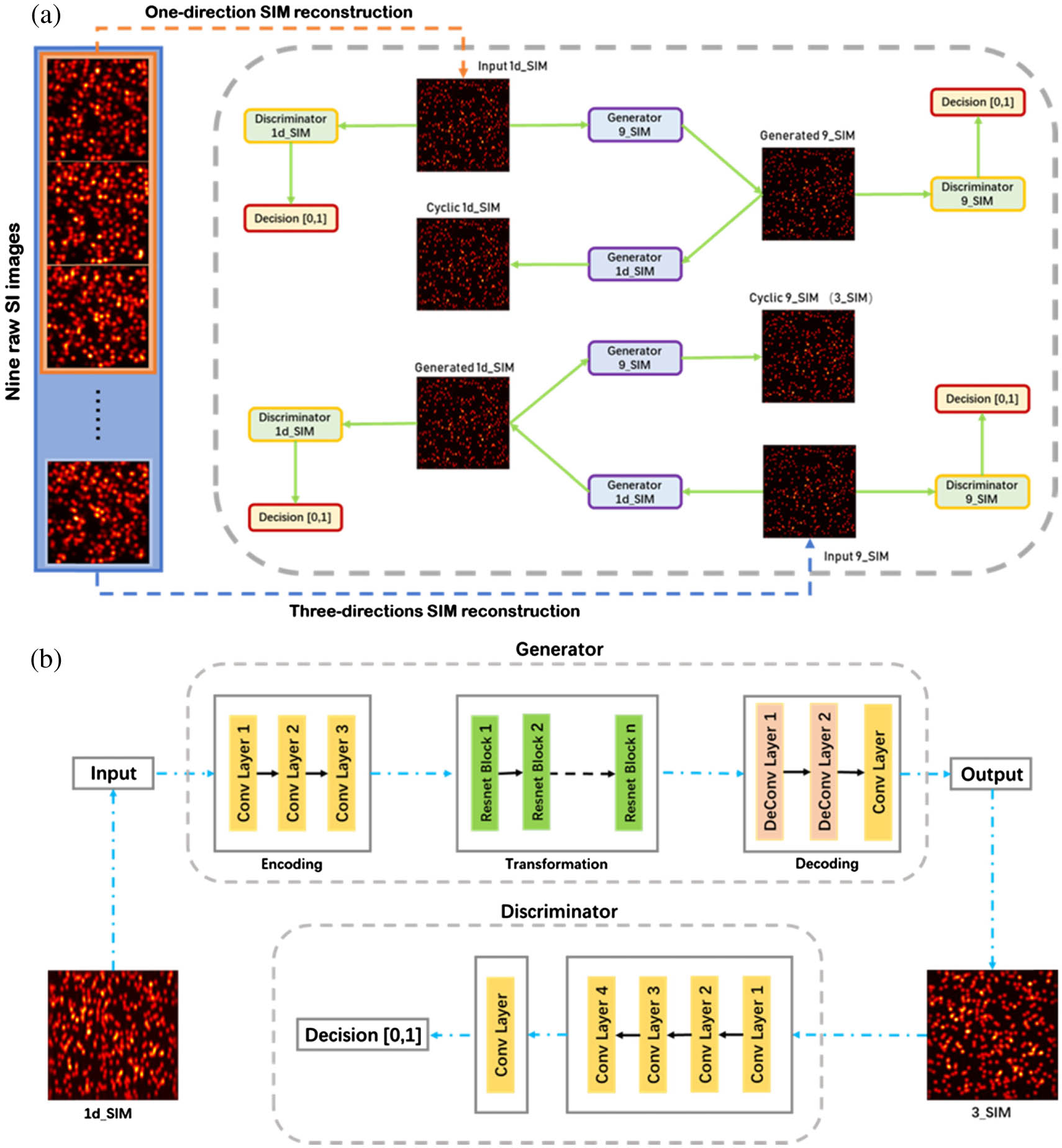
Figure 1.Schematics of the deep neural network trained for SIM imaging. (a) The inputs are 1d_SIM and 9_SIM images generated by nine lower-resolution raw images (using the SIM algorithm) as two training datasets with different training labels. The deep neural network features two generators and two discriminators. These generators and discriminators are trained by optimizing various parameters to minimize the adversarial loss between the network’s input and output as well as cycle consistency loss between the network’s input image and the corresponding cyclic image. The cyclic 9_SIM in the schematics is the final image (3_SIM) desired. (b) Detailed schematics of half of the CycleGAN training phase (generator 1d_SIM and discriminator 9_SIM). The generator consists of three parts: an encoder (which uses convolution layers to extract features from the input image), a converter (which uses residual blocks to combine different similar features of the image), and a decoder (which uses the deconvolution layer to restore the low-level features from the feature vector), realizing the functions of encoding, transformation, and decoding. The discriminator uses a 1D convolution layer to determine whether these features belong to that particular category. The other half of the CycleGAN training phase (generator 9_SIM and discriminator 1d_SIM) is the same as this.
Discriminator A and discriminator B input images of the 1d_SIM and 9_SIM datasets, respectively, are trained by the loss function to identify the generated image as one output by the generator. If the discriminator recognizes it as such, the input image is rejected. If generators A and B want to ensure that the images they generate are accepted by the discriminator, the generated images need to be very close to the original image. This can be implemented using . The discriminator also needs to be upgraded so that the discriminator can determine whether the output image is a raw image or one generated by the generator.
3. RESULTS
We validated the proposed method on both simulated and experimental data. To enable quantitative comparison, the 1d_SIM and 9_SIM images were generated from the same raw datasets. The 1d_SIM images were reconstructed from three of the nine raw SI frames, and the 9_SIM images were reconstructed from all nine raw SI frames. To verify the effectiveness of the neural network on images with different features, the authors prepared three datasets for training containing points, lines, and curves.
All datasets were generated in MATLAB. First, we generate some pixel size random binary images, superposed illuminating patterns and convolved with the point diffusion function (PSF), and we obtain nine raw no-noise SI images. Each pixel represents 10 nm; the PSF is based on the first-order Bessel function, where NA is set to 1.5 and wavelength is set to 532 nm; the pattern vector is 18; and the modulation index is 0.8. We reconstruct these raw SI images by SIM algorithm [37]; for three raw SI images in the same pattern direction we get the 1d_SIM image, and for all nine raw SI images we get the 9_SIM image. Using the 1d_SIM and 9_SIM images as image pairs for the datasets, a total of 2000 image pairs were obtained for training, 200 image pairs for validation, and 200 image pairs for testing. All these simulated image reconstructions were obtained on a grid with a pixel size of 10 nm. The network was then trained using the 9_SIM and 1d_SIM images as inputs. After 10,000 iterations, models trained on the datasets of points, lines, and curves were obtained. All training was performed on the cloud server Intel Xeon E5-2650L, with 64 GB of RAM and NVIDIA GeForce RTX 2080Ti, for 3 h using the TensorFlow framework. Once the network had been trained, reconstructing a image required only 10 s on an office computer.
The trained model was applied to a distinct set of SIM images generated by the same stochastic simulation. First, model performance was tested on the dataset of point images (Fig. 2). A total of 400 points were randomly distributed over the images. Because of a lack of high-frequency information in the direction, the shape of the points in the 1d_SIM image dataset was oval [Fig. 2(b)], and some closely spaced points could not be distinguished in this direction. Figure 2(c) shows that the neural network successfully resolved the issue of the closely spaced points, providing a good match for the 9_SIM images [Fig. 2(d)]. Similarly, points that could not be distinguished in the direction of the 1d_SIM images were rendered distinguishable. Figure 2(e) shows the full width at half-maximum (FWHM) of the points in each image, and we can see that the neural network (3_SIM) can achieve a resolution similar to that of the traditional SIM method (9_SIM).

Figure 2.Experimental comparison of imaging modes with a database of point images. For all methods, nine raw SI images were used as the basis for processing. (a) The WF image was generated by summing all raw SI images. (b) 1d_SIM images were generated by three raw SI images in the direction. (c) The 3_SIM images formed the output of the CNN training. (d) 9_SIM image reconstructed from nine SI raw images as the ground truth. The enlarged area shows neighboring beads in the dashed box. In both the 3_SIM and the 9_SIM images, the beads are distinguishable and yield a resolution beyond the diffraction limit, which 1d_SIM images cannot realize. The resolution of the point is shown in (e).
To further quantify this improvement in resolution achieved by the CNN, complex graphics were used to test the proposed method. Figure 3 shows the training results of the proposed method on the dataset of lines. Each image contained 50 straight lines with different slopes. Using the pretrained deep neural network and inputting the 1d_SIM images [Fig. 3(b)], images with enhanced resolutions were generated as shown in Fig. 3(c). A number of features were clearly resolved in the network output, providing very good agreement with the ground truth (9_SIM) images shown in Fig. 3(d). In Fig. 3(e), we can see that in the lines image, the neural network can still achieve the same resolution as SIM.
Figure 3.Using deep learning to transform images in the dataset of lines from 1d_SIM to 9_SIM. (a) WF line image. (b) 1d_SIM line image used as network input. (c) 3_SIM line image used as network output. (d) 9_SIM line image used as contrast. (e) The achieved resolution of different approaches of line images.
Figure 4 shows the training results of the proposed method on the dataset of randomly generated curves. After the training phase, the neural network blindly took an input image [1d_SIM, Fig. 4(b)] and output a super-resolved 3_SIM image [Fig. 4(c)] that matched the 9_SIM image [Fig. 4(d)] of the same sample. The resolution of the image was significantly improved (as shown in the dotted box).
Figure 4.Deep learning-enabled transformation of images of curves from 1d_SIM to 9_SIM. (a) WF curve image. (b) 1d_SIM image of curves used as input to the neural network. (c) 3_SIM image that was the network output, compared to the (d) 9_SIM image.
The proposed method was also tested on a homemade setup of total internal reflection structured illumination microscopy (TIRF-SIM) shown in Fig. 5. Large datasets are typically used to train a deep neural network, but obtaining massive amounts of experimental images is challenging. A large dataset was obtained here by cutting the experimental images.
Figure 5.Experimental setup for the TIRF-SIM. A laser beam with a wavelength of 532 nm was employed as the light source. After expansion, the light was illuminated into digital micromirror device (DMD) and generated structured illumination. A polarizer and a half-wave plate were used to rotate the polarization orientation; a spatial mask is used to filter the excess frequency components. The generated structured illumination is tightly focused by a high-numerical-aperture (NA) oil-immersion objective lens (Olympus, , ) from the bottom side onto the sample. The sample was fixed at a scanning stage and was prepared with the following procedures. A droplet of dilute nanoparticles (100 nm, attached with R6G molecules) suspension was subsequently dropped onto the prepared cover slip and evaporated naturally. After rinsing with water and air drying, the sample was ready for use.
Fluorescent beads [labeled with Rhodamine 6G (R6G) molecules, Bangs Laboratories] with a nominal diameter of 100 nm were imaged using a SIM system. The microscope was equipped with an oil-immersion objective lens. (Olympus, , ), and the excitation light was 532 nm. The peak wavelength of emission of fluorescence was 560 nm. An sCMOS (scientific complementary metal oxide semiconductor) camera (Hamamatsu, ORCA-flash 3.0) was used, with each pixel representing 65 nm in the sample plane.
Images of size were used in the experiment. The SIM algorithm (fairSIM ImageJ plugin [38]) was used to obtain the 1d_SIM and 9_SIM images. We cropped the images in the center area for each SIM image where there were the most fluorescence points. Then these images were cropped into smaller regions: size images every 256 pixels. Finally, 16 image pairs were obtained for each raw SIM image pair, and a total of 6816 image pairs for 426 raw SIM image pairs. A total of 3000 image pairs were filtered out as the training dataset, 200 as the validation dataset, and 200 image pairs as the testing dataset. The exposure time of each SIM picture is 200 ms, and each pixel in the cropped image represents 32.5 nm. The NA of the objective lens and the wavelength of the laser are consistent with the simulation, and the average modulation index of the pattern is 0.4.
The training model was obtained after 10,000 iterations, and then we applied it to the 1d_SIM nanoparticles’ test data. As shown in Fig. 6(b), some of the nanobeads in the samples were closely spaced. The 1d_SIM image could be super-resolved in only one direction; the other directions, within the classical diffraction limit, that is, under therefore could not be resolved in the 1d_SIM images. After network reconstruction, these closely spaced nanoparticles were resolved in all directions [Fig. 6(c)], and the resulting picture was consistent with that of the 9_SIM images [Fig. 6(d)] in the same regions of the sample. As seen in the line chart on the right of Fig. 6, deep learning achieves a similar resolution to SIM, and both can separate the center distance from the two points of 195 nm and 162 nm.
Figure 6.Comparison of the experiment results of deep learning [(c) 3_SIM]) with (a) WF, (b) 1_direction SIM, and (d) 9_SIM. Wide-field images were generated by summing all raw images, 1d_SIM images were reconstructed using three SI raw images in one direction (), and the 9_SIM images were reconstructed from all nine SI raw images and used as ground truth compared with the 3_SIM images. The 1d_SIM image was used as input to the network to generate the 3_SIM images. The dotted frame in the figures shows an enlarged view of two areas (A and B), where the intensity distribution of the white dotted line is shown in the line chart on the right. In (a), two closely spaced nanobeads that could not be resolved by TIRF microscopy, and the 1d_SIM image super-resolved in one direction in (b). The trained neural network took the 1d_SIM image as input and resolved the beads, agreeing well with the SIM images.
For a quantitative assessment of the quality of the images output by the network, the corresponding root mean square error (RMSE), peak signal-to-noise ratio (PSNR), structural similarity (SSIM index) [39], and mean structural similarity index (MSSIM) [40] were computed as shown in Table 1. The SSIM and MSSIM correlated well with judgments based on the human visual perception. These indices were used to evaluate the differences between the images output by the network and the 9_SIM images. For any kind of images, the difference between the network’s output and the 9_SIM image was minor. This shows that the proposed method is effective at SIM imaging. The number of images needed to achieve the same resolution as traditional SIM imaging was reduced.
| Method | RMSE | PSNR | SSIM | MSSIM |
| Point (simulated) | 7.4610 | 30.7772 dB | 0.9796 | 0.9387 |
| Line (simulated) | 5.3098 | 30.6402 dB | 0.9772 | 0.9291 |
| Curve (simulated) | 7.7903 | 28.4899 dB | 0.9660 | 0.8989 |
| Nanoparticles (real) | 6.9316 | 28.7126 dB | 0.9297 | 0.8347 |
Table 1. Performance Metrics of the Proposed Method on the Testing Data
Deep learning can also be used to transform images from wide field (WF) to SIM [41], but the proposed method has shortcomings. In WF-to-SIM transformation (WF2SIM), the high-frequency information is completely recovered through the guess of the neural network. But in 1d_SIM-to-SIM transformation (1d_SIM2SIM), some high-frequency information already exists in the image, and the neural network does not completely recover the high-frequency information by guessing. The WF2SIM method was compared with the 1d_SIM2SIM method, and we proved the superiority of the latter.
As shown in Fig. 7(a), assuming that the fluorescent luminescence was isotropic and the distribution of intensity of the light source was Gaussian, its Fourier transform was also Gaussian and the spectral distribution was highly symmetric. In particular, this assumption can be guaranteed at the spatial resolution of SIM because it () is higher than the size of the fluorescent molecules (). The final fluorescence belonged to fluorescence group luminescence. In fluorescence imaging, the samples were labeled according to the fluorescent molecules, and the final images represented the total luminescence of a large number of fluorescent groups. This corresponded with the spatial spectral plane, which was also the spatial spectral superposition of all fluorescent groups. Owing to the symmetry of the spatial spectrum of a single fluorescent group, the spectrum of the final images featured high spatial association as shown in Fig. 7(a).
Figure 7.Fourier analysis of the reconstructed images. (a) Comparison of the frequency spectrum of images with different numbers of Gaussian points. The frequency spectrum of the Gaussian points is highly symmetrical. (b) The different colors indicate different types of frequency-related information. The yellow area represents the frequency-related information of the original image, and the green area represents information restored by the network. The grid in (b) represents the relationship between the available frequency-related information and the frequency-related information recovered by the network. (c) The Fourier transform of the reconstructions in Fig. 2 was used to obtain the spectra. To illustrate the Fourier coverage of each model, three circles are marked in each image, where the green–yellow circle corresponds to support for the WF image, the blue circle corresponds to that for the 1d_SIM image, and the yellow circle represents support for the 3_SIM and 9_SIM images.
We calculate the correlation of the spectrum information with a length of ( is the OTF cutoff frequency) in the direction and the direction (see Data File 1). All the calculated correlation coefficients are between 0.5 and 0.8, so the two segments of 1D spectrum information in the -axis and -axis directions can be considered to be significantly correlated. If two pieces of information are related, then they must not be independent. Therefore, the spectrum information in all directions (for example, on the axis and axis) is highly related. Characteristics of the spatial spectral correlation of the fluorescent groups on the spatial spectral plane were determined using CNNs. Then, based on the one-dimensional high-precision spatial spectrum measured, we can use CNNs to extend the two-dimensional high-precision spatial spectrum, which can reconstruct high-resolution image of SIM.
In the process of WF2SIM, the network was used to recover high-frequency information in the image [Fig. 7(b)]. Although the output image was highly consistent with the target image, it lacks a certain degree of credibility in theory because the high-frequency information was completely estimated by the neural network.
In the 1d_SIM2SIM process, some high-frequency information was already present in the images [Fig. 7(c)] and was recovered by the frequency shift in SIM. Because of the high symmetry of the spectrum, this high-frequency information was also available in other directions. To better visualize the recovered high-frequency information, the results are presented in Fourier space. The spectrum of the WF image was mostly concentrated in the green dotted line region, the 1d_SIM algorithm expanded the spectrum in the direction (blue dotted line region), and the 9_SIM expanded the spectrum in all three directions (yellow dotted line region). The image following neural network processing expanded the spectrum, which became nearly consistent with 9_SIM.
Different models were trained using different numbers of data items for the WF2SIM and 1d_SIM2SIM training datasets, and they were used to reconstruct the WF and 1d_SIM images, respectively. Figures 8(e)–8(h) show the reconstructed WF image where some details were not restored; but in the reconstructed 1d_SIM images, the detail was correctly reconstructed [Figs. 8(b) and 8(c)]. In Figs. 8(i) and 8(j), transformations of the loss functions of the generator and cyclic consistency by the neural network are shown. The curve of the loss function of 1d_SIM converged more easily, whereas that of the WF struggled to converge, indicating the uncertainty in the recovery process of the WF image. Hence, 1d_SIM can better recover image detail and train the network model more efficiently, even though it requires two more images.
Figure 8.Comparing WF to 9_SIM with 1d_SIM to 9_SIM. (a) The 9_SIM image reconstructed from nine SI raw images. (b)–(d) Network output, 200, 500, and 900 image pairs (1d_SIM and 9_SIM) were used to train the network models, respectively. (e)–(h) Network output, using 100, 200, 500, and 900 image pairs (WF and 9_SIM) as datasets to train the network models. Each network underwent 10,000 iterations. Some details were not correctly restored in the WF-to-9_SIM training model. The arrows in (a)–(h) point to a missing detail.
4. CONCLUSION
Since the introduction of structured illumination microscopy, numerous algorithms have been developed to reconstruct super-resolved images from SI images. Considerable effort has been invested to reduce the number of raw SI frames, but images generated by such treatment are poor and require parameter tuning.
This study proposed a fast, precise, and parameter-free method for super-resolution imaging using SI frames. Unpaired simulated SIM images were used for unsupervised training by the CycleGAN network. The results of experiments showed that the CycleGAN used in this work performed well to help generate a reconstructed SIM image from three raw SIM frames (3_SIM). The quality of the generated image was very similar to the original nine-frame SIM image (9_SIM). The image reconstructed using 1d_SIM images through CNNs yielded images of better quality than that reconstructed from the WF image. During network training, 1d_SIM to 9_SIM also delivered better performance. In addition, recent studies [42] have shown that the frames in SIM can also be reduced by using U-net, and achieve super-resolution imaging with reduced photobleaching. However, in this method, U-net training requires a large amount of computing resources, so the training efficiency is far less than that of the CycleGAN used in this paper.
The central idea of the proposed technique is based on the observation that the SI image datasets contained a large amount of structural information. By the principle of ergodicity, statistical information learned from such large datasets ensembles in a 1d_SIM image is sufficient to predict 9_SIM images with high fidelity.
All images were blindly generated here by the deep network: that is, the input images were not previously seen by the network. Thus, the network can recover images by learning missing high-frequency information from large datasets, instead of merely replicating the images.
As a purely computational technique, the proposed method does not require any changes in current systems of microscopy and requires only standard 1d_SIM and 9_SIM images for training. Although different types of images need to be trained separately, the neural network used in our method enables us to complete the training efficiently. Once the model has been trained, it can be applied to new 1d_SIM images to rapidly generate a 9_SIM image. This approach can also be extended to nonlinear SIM to reduce the number of frames needed to render it suitable for bio-imaging.
Acknowledgment
Acknowledgment. L. Du acknowledges the support given by the Guangdong Special Support Program.
References
[1] E. Abbe. Contributions to the theory of the microscope and that microscopic perception. Arch. Microsc. Anat., 9, 413-468(1873).
[2] M. J. Rust, M. Bates, X. Zhuang. Sub-diffraction-limit imaging by stochastic optical reconstruction microscopy (STORM). Nat. Methods, 3, 793-795(2006).
[3] M. Bates, B. Huang, G. T. Dempsey, X. Zhuang. Multicolor super-resolution imaging with photo-switchable fluorescent probes. Science, 317, 1749-1753(2007).
[4] S. T. Hess, T. P. K. Girirajan, M. D. Mason. Ultra-high resolution imaging by fluorescence photoactivation localization microscopy. Biophys. J., 91, 4258-4272(2006).
[5] H. Shroff, C. G. Galbraith, J. A. Galbraith, E. Betzig. Live-cell photoactivated localization microscopy of nanoscale adhesion dynamics. Nat. Methods, 5, 417-423(2008).
[6] M. G. L. Gustafsson, D. A. Agard, J. W. Sedat. Doubling the lateral resolution of wide-field fluorescence microscopy using structured illumination. Proc. SPIE, 3919, 141-150(2000).
[7] M. G. L. Gustafsson, L. Shao, P. M. Carlton, C. J. R. Wang, I. N. Golubovskaya, W. Z. Cande, D. A. Agard, J. W. Sedat. Three-dimensional resolution doubling in wide-field fluorescence microscopy by structured illumination. Biophys. J., 94, 4957-4970(2008).
[8] T. A. Klar, S. Jakobs, M. Dyba, A. Egner, S. W. Hell. Fluorescence microscopy with diffraction resolution barrier broken by stimulated emission. Proc. Natl. Acad. Sci. USA, 97, 8206-8210(2000).
[9] E. Betzig, G. H. Patterson, R. Sougrat, O. W. Lindwasser, S. Olenych, J. S. Bonifacino, M. W. Davidson, J. Lippincott-Schwartz, H. F. Hess. Imaging intracellular fluorescent proteins at nanometer resolution. Science, 313, 1642-1645(2006).
[10] H. Linnenbank, T. Steinle, F. Morz, M. Floss, C. Han, A. Glidle, H. Giessen. Robust and rapidly tunable light source for SRS/CARS microscopy with low-intensity noise. Adv. Photon., 1, 055001(2019).
[11] P. Fei, J. Nie, J. Lee, Y. Ding, S. Li, H. Zhang, M. Hagiwara, T. Yu, T. Segura, C.-M. Ho, D. Zhu, T. K. Hsiai. Subvoxel light-sheet microscopy for high-resolution high-throughput volumetric imaging of large biomedical specimens. Adv. Photon., 1, 016002(2019).
[12] E. Narimanov. Resolution limit of label-free far-field microscopy. Adv. Photon., 1, 056003(2019).
[13] E. F. Fornasiero, K. Wicker, S. O. Rizzoli. Super-resolution fluorescence microscopy using structured illumination. Super-Resolution Microscopy Techniques in the Neurosciences, 133-165(2014).
[14] M. G. L. Gustafsson. Nonlinear structured-illumination microscopy: wide-field fluorescence imaging with theoretically unlimited resolution. Proc. Natl. Acad. Sci. USA, 102, 13081-13086(2005).
[15] F. Orieux, E. Sepulveda, V. Loriette, B. Dubertret, J.-C. Olivo-Marin. Bayesian estimation for optimized structured illumination microscopy. IEEE Trans. Image Process., 21, 601-614(2012).
[16] S. Dong, J. Liao, K. Guo, L. Bian, J. Suo, G. Zheng. Resolution doubling with a reduced number of image acquisitions. Biomed. Opt. Express, 6, 2946-2952(2015).
[17] A. Lal, C. Shan, K. Zhao, W. Liu, X. Huang, W. Zong, L. Chen, P. Xi. A frequency domain SIM reconstruction algorithm using reduced number of images. IEEE Trans. Image Process., 27, 4555-4570(2018).
[18] F. Strohl, C. F. Kaminski. Speed limits of structured illumination microscopy. Opt. Lett., 42, 2511-2514(2017).
[19] W. H. Richardson. Bayesian-based iterative method of image restoration. J. Opt. Soc. Am., 62, 55-59(1972).
[20] M. Ingaramo, A. G. York, E. Hoogendoorn, M. Postma, H. Shroff, G. H. Patterson. Richardson-Lucy deconvolution as a general tool for combining images with complementary strengths. Chem. Phys. Chem., 15, 794-800(2014).
[21] M. I. Jordan, T. M. Mitchell. Machine learning: trends, perspectives, and prospects. Science, 349, 255-260(2015).
[22] Y. LeCun, Y. Bengio, G. Hinton. Deep learning. Nature, 521, 436-444(2015).
[23] A. Krizhevsky, I. Sutskever, G. E. Hinton. ImageNet classification with deep convolutional neural networks. Commun. ACM, 60, 84-90(2017).
[24] Y. Rivenson, Z. Gorocs, H. Gunaydin, Y. Zhang, H. Wang, A. Ozcan. Deep learning microscopy. Optica, 4, 1437-1443(2017).
[25] W. Ouyang, A. Aristov, M. Lelek, X. Hao, C. Zimmer. Deep learning massively accelerates super-resolution localization microscopy. Nat. Biotechnol., 36, 460-468(2018).
[26] E. Nehme, L. E. Weiss, T. Michaeli, Y. Shechtman. Deep-STORM: super-resolution single-molecule microscopy by deep learning. Optica, 5, 458-464(2018).
[27] N. Thanh, Y. Xue, Y. Li, L. Tian, G. Nehmetallah. Deep learning approach to Fourier ptychographic microscopy. Opt. Express, 26, 26470-26484(2018).
[28] Z. Ghahramani, I. J. Goodfellow, J. Pouget-Abadie, M. Welling, C. Cortes, M. Mirza, N. D. Lawrence, B. Xu, D. Warde-Farley, K. Q. Weinberger, S. Ozair, A. Courville, Y. Bengio. Generative adversarial nets. Proceedings of the 27th International Conference on Neural Information Processing Systems, 2672-2680(2014).
[29] , J.-Y. Zhu, T. Park, P. Isola, A. A. Efros. Unpaired image-to-image translation using cycle-consistent adversarial networks. IEEE International Conference on Computer Vision, 2242-2251(2017).
[30] M. Mirza, S. Osindero. Conditional generative adversarial nets(2014).
[31] L. A. Gatys, A. S. Ecker, M. Bethge. Image style transfer using convolutional neural networks. Proceedings of the IEEE Conference on Computer Vision and Pattern Recognition (CVPR), 2414-2423(2016).
[32] , P. Isola, J.-Y. Zhu, T. Zhou, A. A. Efros. Image-to-image translation with conditional adversarial networks. 30th IEEE Conference on Computer Vision and Pattern Recognition, 5967-5976(2017).
[33] B. Leibe, C. Li, J. Matas, M. Wand, N. Sebe, M. Welling. Precomputed real-time texture synthesis with Markovian generative adversarial networks. Computer Vision—European Conference on Computer Vision (ECCV), 702-716(2016).
[34] K. Daniilidis, N. Sundaram, T. Brox, P. Maragos, K. Keutzer, N. Paragios. Dense point trajectories by GPU-accelerated large displacement optical flow. Computer Vision—European Conference on Computer Vision (ECCV), 438-451(2010).
[35] , C. Godard, O. Mac Aodha, G. J. Brostow. Unsupervised monocular depth estimation with left-right consistency. 30th IEEE Conference on Computer Vision and Pattern Recognition (CVPR), 6602-6611(2017).
[36] , K. He, X. Zhang, S. Ren, J. Sun. Deep residual learning for image recognition. IEEE Conference on Computer Vision and Pattern Recognition (CVPR), 770-778(2016).
[37] A. Lal, C. Shan, P. Xi. Structured illumination microscopy image reconstruction algorithm. IEEE J. Sel. Top. Quantum Electron., 22, 6803414(2016).
[38] M. Mueller, V. Moenkemoeller, S. Hennig, W. Huebner, T. Huser. Open-source image reconstruction of super-resolution structured illumination microscopy data in ImageJ. Nat. Commun., 7, 10980(2016).
[39] Z. Wang, A. C. Bovik, H. R. Sheikh, E. P. Simoncelli. Image quality assessment: from error visibility to structural similarity. IEEE Trans. Image Process., 13, 600-612(2004).
[40] M. B. Matthews, Z. Wang, E. P. Simoncelli, A. C. Bovik. Multi-scale structural similarity for image quality assessment. Conference Record of the 37th Asilomar Conference on Signals, Systems & Computers, 1398-1402(2003).
[41] H. Wang, Y. Rivenson, Y. Jin, Z. Wei, R. Gao, H. Gunaydin, L. A. Bentolila, C. Kural, A. Ozcan. Deep learning enables cross-modality super-resolution in fluorescence microscopy. Nat. Methods, 16, 103-110(2019).
[42] L. Jin, B. Liu, F. Zhao, S. Hahn, B. Dong, R. Song, T. C. Elston, Y. Xu, K. M. Hahn. Deep learning enables structured illumination microscopy with low light levels and enhanced speed. Nat. Commun., 11, 1934(2020).


