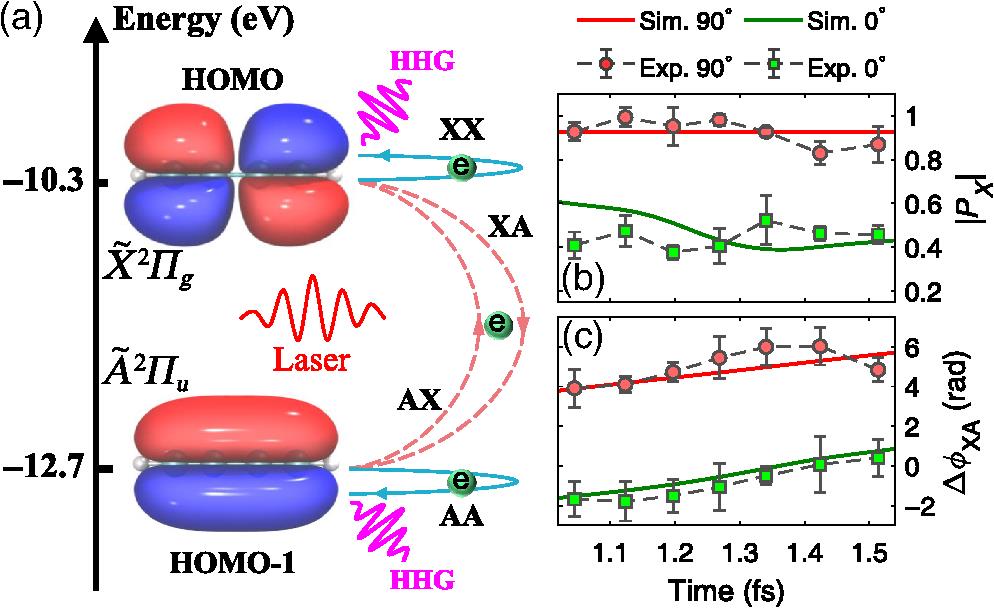
Fig. 1. Probing CM in C4H2 with HHS. (a) Schematic layout of the multichannel HHG in C4H2 molecule that involves the ground X˜2Πg (X˜) and first excited states A˜2Πu (A˜) of the molecular ion. In C4H2, there are four channels labeled as XX, AA, XA, and AX, respectively, contributing to HHG. Here the first and second letters label the ionic state after ionization and before recombination, respectively. (b), (c) Experimentally retrieved population amplitude (|PX|) of the X˜ state (b) and the relative phase (ΔϕXA) between the wave functions of X˜ and A˜ states (c) for the parallel (0 deg, green squares) and perpendicular (90 deg, red circles) alignment of the C4H2 molecule. The solid lines show the TDDFT results for comparison. Error bars in panels (b) and (c) represent the SDs of the reconstructions, which are estimated from the experimental errors of the HHG signals with the bootstrap method.

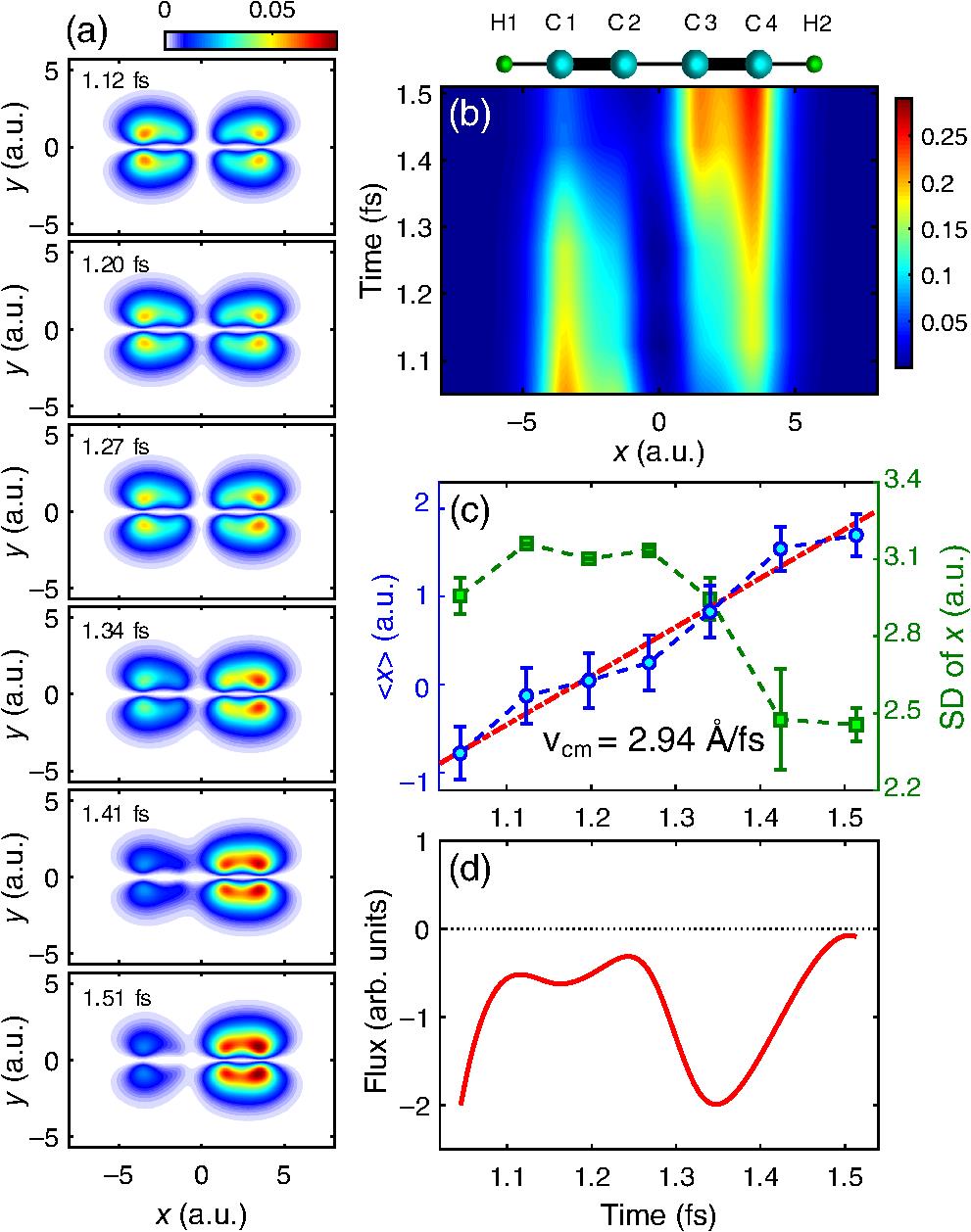
Fig. 2. Reconstruction of CM in C4H2+ for perpendicular alignment. (a) Snapshots of the reconstructed hole densities for the alignment angle of 90 deg. (b) Time-dependent hole densities along the molecular backbone obtained by integration over the y direction. For clarity, the molecular backbone has been plotted on the top of panel (b). (c) Time-dependent COC position ⟨x⟩(t) (dashed line with circles) retrieved from the hole densities in (b). Here the dashed-dotted line is a linear fitting of ⟨x⟩(t) to evaluate the CM speed, and the green squares represent the SD of the x coordinate. (d) Flux of charge density crossing the x=0 plane. Negative value means CM from −x side to +x side.

Fig. 3. Reconstruction of CM in C4H2+ for parallel alignment. (a)–(d) The same as Fig. 2(a)–2(d), but for the case of parallel alignment of the C4H2 molecule.

Fig. 4. TDDFT simulations of the CM dynamics in C4H2+. (a), (b) TDDFT calculations of the reduced hole density ρx(t) and COC position ⟨x⟩(t) in the experimental temporal range for the 90 deg alignment of the C4H2 molecule. (c), (d) Same as panels (a) and (b), but for the parallel alignment (the alignment angle of 0 deg) of the C4H2 molecule.

Fig. 5. Reconstruction of the CM speed in C4H2+. Dashed line with squares shows the CM speed retrieved as a function of the alignment angles. The solid line plots the TDDFT result for comparison.