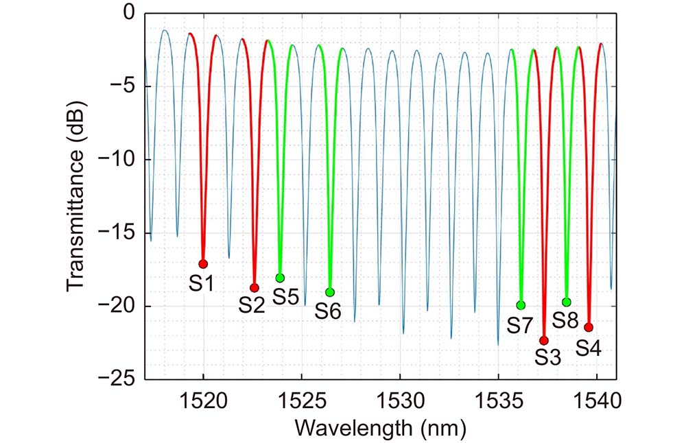
Fig. 1. Transmission spectrum of the S-polarized TFBG before starting the deposition. The 8 resonances that are employed in the method described in the results section are marked (in red for the resonances of modes with even azimuthal order, in green for resonances with odd azimuthal order).

Fig. 2. Schematic diagram of the setup employed in the deposition.

Fig. 3. (a) Experimental shift of the 8 TFBG resonances employed in the proposed method. Resonances S1 - S4 (top row) correspond to even azimuthal orders, and resonances S5 - S8 (bottom row) correspond to odd azimuthal orders. (b) Evolution of the spectrum in the 1515 - 1545 nm range during the deposition.

Fig. 4. Graphical representation of how to obtain the deposition rate that best fits the experimental with the simulated data for each n value. Here, the experimental wavelength shift of resonance S1 and the simulated data for n = 2.00 and n = 2.48 are used.

Fig. 5. Graphical explanation on how to calculate the time instant that minimizes the total error for the 8 resonances for a certain simulated (n, T) point. In this example, (n = 2.20, T = 100 nm), and the error is graphically shown for t_i = 150 min.

Fig. 6. (a) Fitted (n, T, t_fitted) points plotted in a thickness vs. time graph for n = 2.00, n = 2.20, and n = 2.48. (b) Final thickness obtained for each n value with the proposed method.

Fig. 7. Mean wavelength error per resonance over all thicknesses (ε_global(n)) for each tested index value (n).

Fig. 8. (a) Simulated wavelength shift for S1 for n values between 2.00 and 2.48 (0.04 steps) and different thicknesses that vary depending on the n value. (b) Experimental wavelength shift of S1 during the deposition.

Fig. 9. Second iteration results. (a) Mean wavelength error per resonance (ε_global(n)) over all thicknesses for each tested index value (n). (b) Final thickness obtained for each n value with the proposed method. In both graphs the optimum solution is marked with a green star and (b) includes an inset that shows how the error in the n value of the solution is calculated.

Fig. 10. Dispersion curve for n measured by the ellipsometer on a thin film on a witness sample.

Fig. 11. FESEM images in which the thin film thickness is measured in the TFBG cross-section.

Table 0. Results for the 1^st iteration of the proposed method and thickness selection for the 2^nd iteration.

Table 0. Comparison between the proposed method, the ellipsometer and the FESEM.