Measuring the refractive index and the thickness of thin films (films with a thickness from less than a nanometer to several microns) is essential to characterize them¹, and improve the performance of sensors and devices that employ thin films. The most established method to simultaneously determine both parameters, with a wide range of available commercial solutions, is ellipsometry. Ellipsometry is based on measuring the changes in the state of polarization of light after its reflection on the sample whose thickness and refractive index are unknown. The sample must be placed on a substrate whose refractive index is known. The incident light has a known polarization state, and the reflected light is elliptically polarized (thus the name of the technique), being characterized by the following equation^2-4:

ρ=rprs=tan(Ψ)⋅eiΔ,（1）

where ρ is the ratio of the reflection coefficients rp (corresponding to P-polarized light) and rs (corresponding to S-polarized light), and Ψ and Δ are known as the ellipsometric angles, and they are defined as the amplitude ratio (Ψ) and the phase difference (Δ), respectively. Ψ and Δ depend on the substrate, the wavelength and angle of the incident light, and the refractive index and thickness of the thin film deposited on the substrate⁴. When several incident wavelengths are used, the technique is known as spectroscopic ellipsometry, and it is one of the dominant ellipsometric techniques nowadays as it allows to measure the dispersion of refractive indices with wavelengths^{1, 3}.

The main advantages of ellipsometry include its high sensitivity, and being a nondestructive and contactless method³. The most important drawback of ellipsometry is that the refractive index and the thickness cannot be directly deduced from Ψ and Δ, unless the sample is very thick and can be considered an isotropic bulk material. An optical model of the thin film material is required, and the thickness and refractive index are determined through a fitting process between this optical model and the measurements carried out by the ellipsometer.

Another commercially available method to measure both the thickness and the refractive index of thin films is spectroscopic reflectometry. It is an interferometric technique consisting in measuring the reflected light from the sample along a broad range of wavelengths. The light reflected at the different interfaces (air/thin film, and thin film/substrate) interferes, and the optical path difference depends on the thickness of the thin film. This technique calculates the thickness and the refractive index by comparing the experimental measurements with the ones obtained through simulations for assumed values of these parameters, until a good fitting is achieved through an iterative process¹.

In the research field, another conventional method is based on using a prism coupler^5-8, and consists in coupling light to a thin film deposited on the prism, exciting several modes, which are then coupled out of the thin film and projected on a screen, creating a pattern with several lines (called mode lines or m-lines). The angles between these lines and the normal of the prism enable to compute both the thickness and the refractive index of the thin film. The limitation of this method is that it only works with films that have a refractive index higher than that of the substrate and thick enough to support guided modes. In more recent years, different approaches based on interferometry have been proposed: dual wavelength interference^{9, 10}, low-coherence interferometry combined with confocal optics¹¹, or optical coherence tomography¹², among others. Finally, a recently proposed method involves employing surface plasmon resonances in a Kretschmann configuration^13-16.

In this work, we propose a completely different approach to determine the thickness and refractive index of thin films, based on the wavelength shifts of multiple cladding mode resonances in tilted fiber Bragg gratings (TFBGs). While different, the underlying principle is the same as that of all the aforementioned methods, i.e. it consists of comparing measured parameters to those obtained from simulations of the same experimental conditions and finding the film parameters that make the simulated results match the experimental ones with the least amount of error. It is also notable that, unlike many thin film characterization tools, the TFBG can be easily monitored during deposition to control the deposition rate and final thicknesses obtained, simply by connecting it to a spectral interrogation system through a fiber compatible port of the deposition tool.

One of the factors that helps to improve the accuracy of the extraction of index and thickness is the phenomenon of mode transition during the growth of a coating on a fiber. The mode transition was initially demonstrated in the case of the long period gratings (LPGs)¹⁷, although this term was coined later¹⁸. When a thin film whose refractive index is higher than that of the cladding and of the surrounding medium is deposited on the fiber, the effective indices of the cladding modes begin to slightly increase as the thin film becomes thicker. When a certain thin film thickness is reached, the optical field of a high order cladding mode acquires an additional maximum in the radial direction and its effective index increases rapidly in the process, resulting in a reorganization of the remaining cladding modes. In highly multimode systems, such as the cladding of a single mode fiber, cladding modes abruptly change their effective index to a value close to the initial effective index of the immediate lower order cladding mode¹⁹. The immediate consequence of this change is a wavelength shift in the attenuation bands of the LPG²⁰, due to the relationship between the effective index of a cladding mode and the wavelength position of the respective attenuation band, given by the phase matching condition:

λi=(neffcore(λi)−neffcladdingi(λi))⋅Λ,（2）

where λi is the wavelength of the attenuation band (resonance) corresponding to the ith cladding mode, neffcore(λi), neffcladdingi(λi) are the effective indices of the core and the ith cladding mode at λi, and Λ is the grating period.

As the change in the cladding mode effective indices during the mode transition is abrupt, the wavelength shift of the corresponding resonances is also large, which means that the sensitivity to the thin film thickness at this point is high. Furthermore, it has also been demonstrated that during the mode transition there is also an increase in the sensitivity to the surrounding medium refractive index (SRI)¹⁹. Consequently, the mode transition has become a common strategy in LPG based SRI sensors^{21, 22}, chemical sensors²³, or biosensors²⁴ with the purpose of improving the sensitivity.

In the context of TFBGs, mode transitions were recently demonstrated through the deposition of a titanium dioxide (TiO₂)²⁵, and an indium tin oxide (ITO)²⁶ thin films on fibers. It was shown that the mode transition presents different characteristics depending on the polarization state of the core-guided light incident on the TFBG²⁵. Two cases were studied, one with S-polarized input core guided light, and the other with P-polarized light (with the S and P states defined relative to the tilt plane of the grating fringes). In the case in which S-polarized light was employed, the mode transition was more abrupt and occurred at lower thin film thicknesses than in the case where P-polarized light was used (P-polarized input light couples predominantly to cladding modes radially polarized at the fiber while S-polarized input couples to tangentially polarized cladding modes). It is also worth mentioning that for TFBGs, the resonances shift towards longer wavelengths during the mode transition, as opposed to LPGs, where the resonances shift towards shorter wavelengths. This is due to the fact that the phase matching condition for a TFBG is²⁷:

λi=(neffcore(λi)+neffcladdingi(λi))⋅Λ/cosθ,（3）

where the terms have the same meaning as the ones in the LPG phase matching condition and θ is the tilt angle. In the TFBG phase matching condition, there is a plus sign (as opposed to the minus sign in the LPG phase matching condition, Eq. 2), which explains this difference between the mode transition in TFBGs and LPGs.

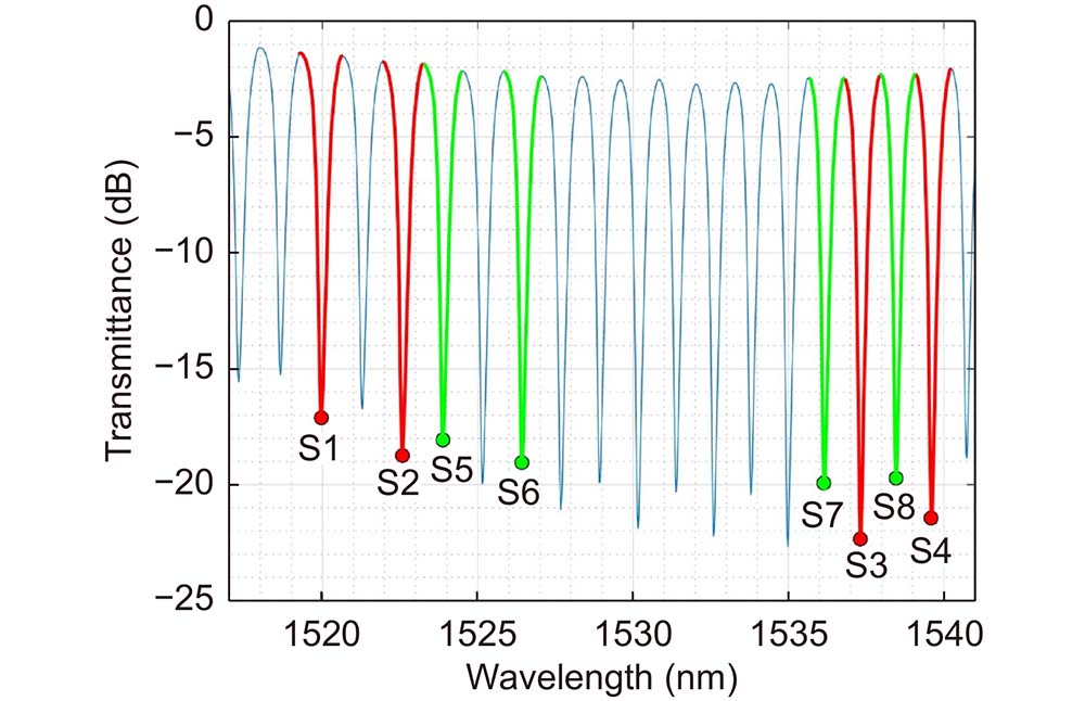
The main reason for using TFBGs in the current work however stems from the fact that cladding mode resonances occur at spectral intervals of the order of 1 nm in typical cases (the spectrum of the TFBG employed in this work is shown in Fig. 1), compared to 10–100 nm in the case of LPGs. This allows simultaneous measurements of a much larger set of cladding mode resonances, each providing a “separate” measurement of the growth of the thin film, as well as a reference wavelength (that of the core mode back reflection) which remains unaffected by the presence and growth of the thin film on the cladding surface. It is these features of the TFBG device which allow sufficient data to be collected during thin film deposition for reducing the uncertainty in the determination of the film parameters through statistical means.

A first step in this direction was obtained in our previous work²⁵. Here, it was demonstrated that the thin film thickness value could be recovered by comparing the experimental and simulated wavelength shift of a single cladding mode resonance during a mode transition, but the simulations required to know the thin film refractive index value, which was measured separately with an ellipsometer. The purpose of the present work is far more ambitious, i.e. to employ the mode transition in TFBGs to recover not only the thin film thickness value, but also its refractive index, thus fully replacing an ellipsometer with fiber optic spectrum measurement tools. It could be argued that the same study could be attempted based on the mode transition in LPGs, but this would require accurate spectral interrogation over a few thousand nm to be able to follow the same number of modes and thus to obtain the same statistical improvement in the accuracy of the extracted film parameters.

The employed TFBG was inscribed over a length of 15 mm on a standard single mode fiber (Corning® SMF-28) with a cladding/core diameter of 125/8 µm. A pulsed KrF excimer laser (PM-800 by Light Machinery) was used to fabricate the grating by the phase mask technique and hydrogen loading of the fiber to enhance its photosensitivity. The core mode resonance was approximately located at 1587 nm, the grating period along the fiber axial direction (Λ/cosθ) was 549 nm, and the tilt angle was 12°. This tilt angle was selected because the cladding modes strongly couple over a wider wavelength range²⁷, thus enabling to monitor the shift of resonances in a broader range. A TiO₂ thin film was deposited uniformly over the whole circumference of the TFBG with the atomic layer deposition technique using a Savannah G2 ALD deposition system (Veeco Inc.), and utilizing ultrapure water and TDMAT (tetrakis(dimethylamido)titanium(IV)) (Sigma-Aldrich S.A) as precursors. The duration of the deposition was approximately 10 h and 21 min (621 min).

In order to monitor the evolution of the TFBG spectrum during the deposition, one end of the fiber was connected to a multi-SLD light source (FiberLabs Inc.), and the other end to an optical spectrum analyzer (HP-86142A from Agilent). This is possible due to the employment of a dome lid with feedthroughs that enable to use fibers to connect the TFBG (inside the ALD chamber), with the measuring equipment. The optical spectrum analyzer was connected to a computer, and the spectrum was acquired and saved at ~25 s intervals. An in-line polarizer (Phoenix Photonics Ltd), and a polarization controller (FPC032 model from Thorlabs Inc.) were placed in the setup between the source and the TFBG to select the S linearly polarized state (relative to the tilt plane) for the core-guided light incident on the TFBG. The P- and S-polarized states can be recognized unambiguously by rotating the input polarization before the deposition since TFBG resonances occur in pairs (in this case, separated by about 0.1 nm) where the resonance at shorter wavelengths corresponds to the P-polarized state and the one at longer wavelengths corresponds to the S-polarized state. The whole setup is depicted in Fig. 2. It was decided to work with the S-polarized state (instead of the P-polarized state) because the mode transition is more abrupt for the S-polarization²⁵, and it was considered that this would help the fitting method proposed in the results section. We note that birefringent films can be measured with this technique since S- and P-polarized modes have perpendicularly oriented electrical fields at the fiber surface. Choosing which modes are used in the analysis allows to measure separately the refractive index in the radial and azimuthal direction (on the surface of the fiber).

The accuracy of the method that is proposed in this work is verified by measuring the refractive index and the thin film thickness with an ellipsometer, and a field-emission scanning electron microscope (FESEM) (in this case, only the thickness). The ellipsometer used is an UVISEL 2 model (Horiba Scientific Thin Film Division) with a spectral range of 0.6–6.5 eV (190–2100 nm), an angle of incidence of 70°, a spot size of 1 mm and software DeltaPsi2™. The sample that was analyzed was a piece of silicon wafer that was placed next to the TFBG inside the ALD chamber during the deposition. The FESEM is an UltraPlus FESEM, from Carl Zeiss, Inc., with an in-lens detector at 3 kV and an aperture diameter of 30 μm. It enables the direct measurement of the thin film thickness on the cross section of the TFBG (which have been cut following the final optical measurements).

The simulations of the TFBG spectrum were performed in MATLAB© using a combination of two algorithms: a fiber mode solver, and a complex coupled-mode program to calculate TFBG transmission spectra²⁸. The mode solver algorithm is based on the finite difference method with a resolution of 3 nm over the 80 µm radius of the calculation window in the radial direction (sufficiently large to assume that the cladding mode fields have decayed to zero beyond the 62.5 µm radius of the fiber) and independent calculations for mode azimuthal orders 0 to 7. The mode solver allows for any number of azimuthally uniform layers in the radial direction, and in particular coatings of any thickness on the cladding surface. The coupled mode approach to calculate transmission spectra²⁹ is modified with several improvements. At each wavelength, 28 modes are calculated (by the mode solver) around an effective index value determined by the requirement of phase matching from the core mode at this wavelength. Then, coupling coefficients for all these modes are determined and the coupled mode equations are solved over the grating length by a Runge-Kutta algorithm.

It is important to note that in order to obtain accurate results, the refractive indices of the core and cladding of the fiber employed in the simulations must be known to the highest possible precision. For the cladding glass, the refractive index values are those of pure silica³⁰, while the core index and dispersion are determined separately by iterative simulations of the measured positions of the resonances of the TFBG used in air (without coating) until the resonance positions match to better than 1 pm on average over the spectral range of interest. This is necessary because the grating fabrication process changes the average refractive index and dispersion of the Germanium-doped core in a manner that varies from grating to grating (at least for the required accuracy, which is of the order of 1 in 10⁶). In the case of the TFBG used in this work, the obtained values for the refractive index of the core material and the dispersion are ncore(λBragg) = 1.450634 and S=0.017036 µm⁻¹, and the refractive index of the core material at each wavelength is then calculated with the following expression: ncore(λ)=ncore(λBragg)+S(λBragg−λ). In the case of the TiO₂ thin film, non-dispersive constant trial values for the real part of the refractive index (n) are assumed (this will be further explained in the results section), while the imaginary part (k) is assumed to be negligible, which is expected for good quality TiO₂. Regarding the surrounding medium (air), a constant value of 1.00027 is used.

Eight resonances are selected to be simulated and compared to the experimental ones. Since TFBGs with relatively small tilt angles couple to modes guided by the cladding and since these modes fill the whole cladding cross-section (with various power distributions associated with their azimuthal orders)²⁷, the use of wavelength shifts from several cladding mode resonances ensures that the measured data provides a reliable representation of the whole coating around the fiber. These 8 resonances have been chosen because they possess a low calibration error (less than 5 pm individually, and less than 0.1 pm on average) in order to increase the accuracy of the method. The calibration error of a resonance is defined as the difference between its experimental wavelength positions before the beginning of the deposition, and the simulated one with the obtained calibration parameters. Out of these 8 resonances, 4 resonances (the ones that are located around 1520.0 nm, 1522.6 nm, 1537.3 nm, and 1539.6 nm at the beginning of the deposition), correspond to even azimuthal orders (m = 0, 2, 4, 6) and the other 4 resonances (initial wavelengths of 1523.9 nm, 1526.4 nm, 1536.2 nm, and 1538.5 nm), to odd azimuthal orders (m = 1, 3, 5, 7). These resonances are denoted from S1 to S8 using the order in which they have been enumerated in the text (S1–S4 correspond to even azimuthal orders, and S5–S8 to odd azimuthal orders). The initial position of these resonances before the beginning of the deposition is shown in Fig. 1, with the even resonances (m = 0, 2, 4, 6) marked in red and the odd resonances (m = 1, 3, 5, 7) marked in green. This choice (i.e. having resonances with even and odd azimuthal orders) has been done to make the proposed method more robust (in case the mode sensitivities would depend somewhat on the parity of the azimuthal order). The experimental shift of these 8 resonances during the deposition is shown in Fig. 3(a). The black line in each graph corresponds to the central wavelength of the respective resonance, which is calculated combining a MATLAB© function for finding peaks and a second order polynomial approximation of the resonance. In order to provide a graphical summary of the experiment, the evolution of all the resonances during the deposition in the 1515–1545 nm range is included in Fig. 3(b), where each of the 8 studied resonances is identified, and its central wavelength shift is also marked with a black line.

The shift of the 8 selected resonances is simulated for values of n of the thin film ranging from 2 to 2.48 in 0.04 steps (13 n values) and for thicknesses T ranging from 0 to 300 nm in 20 nm steps (16T values). The n values employed in the simulation have been selected because the TiO₂ thin film should have a real part of the refractive index in this range based on existing references^{31, 32} and our experience with this material. Once the simulations have been performed, there are two sets of data for each resonance; the experimental wavelength shifts vs. deposition times and the simulated wavelength shifts vs. thickness. The second dataset can be divided in 13 subsets, as there is one subset per each assumed n value of the thin film.

The proposed method has to find in the first place the deposition rate that provides the best fit between the experimental and the simulated data for each n value. This idea is graphically synthesized in Fig. 4, where the time axis (top of the graph) and the experimental wavelength shift of resonance S1 are “stretched” or “compressed” until they fit the simulated data (a video showing this dynamically is included in the Supplementary information). It can be observed in Fig. 4 that deposition rates of 0.42 nm/min and 0.23 nm/min provide good fits for the simulated data with n = 2.00 and n = 2.48, respectively. Another result assuming a 0.30 nm/min deposition rate has also been added for visual comparison. While the correspondence between experiment and simulation visually appears as good for the two index values tested, there are small differences that make it possible to find the “best” value quantitatively, especially when including data from all 8 resonances. It is worth mentioning that Fig. 4 shows that there are some simulated points that cannot be used in the fitting, that is, the ones that correspond to wavelengths shifts higher than the experimental wavelength shift corresponding to the end of the deposition (discontinuous line). This fact has to be taken into account in the proposed method. On the other hand, Fig. 4 only includes the visual fitting of resonance S1, and it is desired to simultaneously fit 8 resonances, in order to obtain a robust method with high accuracy. Based on the previous considerations, the proposed method possesses the following steps:

1) Initial check: all simulated data points (i.e. (n, T) pairs) yielding wavelength shifts larger than the final experimental value (i.e. 1521.9 nm in the case of resonance S1 in Fig. 4) are discarded from the analysis. When n increases, the highest thickness that can be used becomes lower. This is the expected result because, when the thin film value of n is higher, the wavelength shift is faster, requiring thinner thin films to produce the wavelength shift corresponding to the end of the deposition.

2) Fitting: for each (n, T) that verifies the previous condition, it is found the time instant tfitted that minimizes the total error for the 8 resonances. The total error ϵ(n,T,ti) at a certain time instant ti is calculated as the addition of the absolute values of the differences between the simulated and the experimental position of each resonance at that time instant. This error can be expressed with the following formula:

ϵ(n,T,ti)=∑j=18|λj,sim(n,T|−λj,exp(ti)),（4）

where λj,sim(n,T) is the simulated wavelength position for resonance j (with j ∈ [1, 8]) for n and thickness T, and λj,exp(ti) is the experimental wavelength position of resonance j at time instant ti.

An example of how to calculate this error is shown in Fig. 5. These graphs correspond to the case (n = 2.20, T = 100 nm). In each graph (the graph corresponding to S1 has been enlarged for the sake of clarity), the blue line corresponds to the experimental wavelength shift of the respective resonance during the complete deposition, and the black discontinuous line signals the simulated wavelength position of the respective resonance for n = 2.20, T = 100 nm. For ti = 150 min (time instant selected as an example), the green arrows indicate the error for each resonance, and the total error that has to be minimized is the addition of these 8 individual errors. In this case, it can be observed that all the discontinuous black lines cut the experimental shift of the corresponding resonance at approximately ti = 330 min, but the crossing point slightly changes depending on the resonance, so the total error has to be computed to establish which is the “best” time instant tfitted for n = 2.20, T = 100 nm. This process is repeated for all (n, T) points that verified the previous step (“initial check”).

As an additional step, it is checked that for the fitted points (n, T, tfitted), the individual 8 errors for the 8 resonances have a similar order of magnitude. If there had been an outlier resonance with a much higher mean error than all others, it could have been discarded since there is ample remaining data to form a reliable average. This did not occur for this experiment. On the other hand, during this fitting process, no relevant differences have been found between the results obtained with the resonances corresponding to even azimuthal orders and the ones corresponding to odd azimuthal orders. Furthermore, since each resonance is actually made up of at least 4 modes with different azimuthal orders (but almost identical effective indices), this ensures very uniform “probing” of the coating around the fiber circumference.

3) Linearity: the ALD deposition rate is supposed to be constant, but the analysis method proposed here does not assume or need a constant deposition rate. This allows the calculation of a deposition rate vs. time by plotting the thickness vs. time graph and measuring the evolution of the slope. Exemplary fitted (n, T, tfitted) points are plotted in Fig. 6(a) for n = 2.00, n = 2.20, and n = 2.48 values. In all cases (also including the n values that are not represented in Fig. 6(a)), a linear approximation provides an R² value close to 0.99 or even higher, meaning that the deposition rate is essentially constant, as expected for ALD. The final thickness calculated for each n value is shown in Fig. 6(b). The calculated final thickness reduces as the n value increases. As it has been previously mentioned, this is the expected result, as thinner thin films are needed to produce the same wavelength shift as the n value becomes higher.

This way, there are 13 pairs of solutions (n, final T), one per each n value that has been tested. The question that now arises is how to establish which of them is the best one. In order to do this, a global mean error ϵglobal(n) is calculated for each n as the addition of the total error ϵ(n,T,tfitted) made at each fitted point divided by 8 (number of employed resonances), and by the number of employed thicknesses NT(n) for that n value. It has to be remembered that, depending on the tested n value, the number of thicknesses NT(n) that are used is different, so the global error has been defined in a way that compensates this fact. This error can be calculated with the following formula:

ϵglobal(n)=18∑1NT(n)ϵ(n,T,tfitted)NT(n).（5）

The global mean error ϵglobal(n) for each n is plotted in Fig. 7. Nevertheless, there is not a clear minimum (the optimum seems to be in the 2.16–2.40n interval, but it is a very broad range).

However, although precautions have been taken to make a fair comparison between the results for the different n values, the number of thicknesses used varies between index values (13 thicknesses for n = 2, 8 thicknesses for n = 2.48), which may affect the results. In addition to this, it can be argued that there are not enough thickness points for the larger index values.

Based on the results of the first iteration, a second attempt was made with the following differences: for each value of index, a new set of thicknesses were determined such that the number of thicknesses used for each index was equal. In short, the maximum thickness found for each index in Fig. 6(b) was divided into 20 equal intervals as shown in Table 1. Actually, the maximum thickness to be simulated was set a little lower than the final thickness calculated in the first iteration, to make sure that the last thickness simulated would not exceed the final experimental wavelength for all 8 resonances.

The results for this second iteration are shown in Figs. 8, 9 below. Figure 8 shows that all the simulated thicknesses lie below the maximum allowed by the maximum experimental wavelength shift. On the other hand, Fig. 9(a) displays the global mean error calculated for each n value in this second iteration, and Fig. 9(b) provides the new values of the final simulated thicknesses corresponding to each index (they are very similar to those calculated in the first iteration, so it does not make sense to carry out a third iteration). There is a clear minimum at n = 2.24 in Fig. 9(a), but a third order polynomial fit (R² = 0.9626) gives a slightly more precise minimum near 2.25, in spite of apparent slight outliers at n = 2.28, n = 2.44, that do not follow perfectly. It is considered that increasing the number of thickness points in the second iteration (which is the same for each n value) has helped obtain a good fitting and a clear optimum. For n = 2.25, the corresponding final thickness, found from Fig. 9(b) using a second order polynomial fit (R² = 0.9997), is 185 nm. Therefore, the second iteration of the proposed method provides an optimum solution with a thin film index of 2.25 and a final thickness of 185 nm, although the errors still have to be calculated. This n value would be valid in the 1520–1540 nm range, range in which the resonances chosen are located.

In order to calculate the error in the final thickness, the error in the deposition rate can be used. For n = 2.24 (simulated n value closest to n = 2.25), the confidence interval of the deposition rate at 95% confidence level is [0.295, 0.308] nm/min, which corresponds to a [183.2, 191.3] nm interval for the final thickness, that is, an error of around ±4.1 nm. For the rest of tested n values, this error oscillates between ±3.4 nm (n = 2.48) and ±4.6 nm (n = 2.00). Being conservative, an error of ±5 nm can be assumed in the final thickness for any n value. This method for calculating the error in the final thickness would have to be reconsidered in other studies. If the deposition duration increased or the difference between the deposition rates for each n value was larger, the difference between the errors for each n value would be more important (here it is only ±1.2 nm between n = 2.00, and n = 2.48), and perhaps assuming the same error for any n value would not be the best option.

Regarding the error in the n value in the optimum solution, if two lines corresponding to the optimum final thickness ±5 nm are drawn in Fig. 9(b) (see the inset), they cut the (n, final T) curve approximately at n = 2.23 and n = 2.27, so it can be considered that the error in n is ± 0.02. It has to be noted that, with the method employed to calculate the error in n, if the error in the final thickness increased, the error in n would increase too. Therefore, the optimum solution is n = 2.25 ± 0.02, with a final thin film thickness of 185 ± 5 nm. These errors are considered to be acceptable, as they are of the same order of magnitude as the ones given by other conventional methods, as it will be explained in the following.

The validity of the results obtained (n = 2.25, final thickness of 185 nm) can be compared to the values given by traditional means (an ellipsometer and a FESEM). The ellipsometer provides the TiO₂ dispersion curve as well as the thickness of the thin film. The dispersion curve for n is included in Fig. 10, and n = 2.19 ± 0.01 in the TFBG wavelength range (1480–1600 nm) with a thickness value of 178 ± 1 nm. The mean thickness value provided by the FESEM, based on 6 measurements (see Fig. 11), is 183 nm, with a standard deviation of 11 nm.

The obtained results with each method are summarized in Table 2. It can be observed that the final thickness that has been calculated with the proposed method is within 2 nm (or 1.1%) of the physical measurement of the FESEM, while the ellipsometer difference is a little larger (7 nm or 3.9%). Regarding the calculated value for n (n = 2.25 with the proposed method vs. n = 2.19 with the ellipsometer), the difference is 2.7%. It should be pointed out that while ALD is considered a conformal process in the sense that all exposed surfaces in the deposition tool are supposed to be coated similarly, this can also be dependent on the local conditions at each surface: since the fiber and witness samples (for ellipsometric measurements) are not exactly at the same place in the chamber, the differences observed between the fiber and witness samples may be due to actual differences in the films produced. The FESEM does not suffer from this problem since its thickness measurement was carried out on the fiber itself. Therefore, it is considered that the proposed method is reliable and could become an interesting alternative to measure the thickness and refractive index of thin films deposited on fibers in situ and in real time.

Regarding the possible limitations of the proposed method, it is noted that the current demonstration was obtained for a coating that has a higher refractive index than the fiber cladding (~2.2 vs. 1.44 at the wavelengths used) and therefore that a mode transition phenomenon enhances the nonlinearity of the wavelength shift curves. This helps produce better defined minima in the simulation vs experimental shift curves and most probably better accuracy. Other materials that produce the mode transition (their refractive index is higher than that of the cladding), and for which this method could be directly applied, include, for instance, indium tin oxide (ITO), tin oxide (SnO₂) or zinc oxide (ZnO). In fact, the mode transition in TFBGs coated with ITO has already been shown²⁶. A similar demonstration remains to be validated for coatings with an index lower than 1.44, such as gold (Au) or silver (Ag). Although the mode transition does not occur for these materials, it is considered that a similar method, based on monitoring the wavelength shift of the resonances during the deposition and comparing them with the simulated ones, could be employed.

In terms of applicability of the present method, several TFBGs with suitable grating periods (therefore covering different wavelength ranges) would be required in order to measure the refractive index over a broader wavelength range. On the other hand, it was not demonstrated how films with complex refractive indices could be measured. While beyond the scope of the current work, it has been shown before that TFBGs can indeed measure losses in coating (in particular films with lossy surface plasmon resonances²⁷), and that transitions induced by lossy modes have been observed frequently in LPGs^33-35.

In this work, a new method, based on simultaneous analysis of multiple resonance wavelength shifts in TFBGs, has been proposed to measure both the thickness and the refractive index of a thin film deposited on a fiber. In particular, it has been applied to a TiO₂ thin film deposited by means of ALD. The method is based on comparing the experimental wavelength shift of the TFBG resonances with the simulated ones obtained for a range of thicknesses and n values. The proposed method easily finds the deposition rate that better fits the experimental results for an assumed value of n. Then, calculating which pair of (n, final thickness) results best fits the experimental results has been demonstrated through a two-step iterative process starting from rough initial guesses of the expected ranges of the film thickness and index. For routine analysis of similar coatings in production, for instance, the search range would likely be much better known and a single iteration could be sufficient.

It is to be noted that the whole process can be automated (from data gathering to peak fitting and processing): it was carried out using MATLAB© as a set of individual programs but given the human intervention steps we used, there does not appear to be issues into combining those into a single software package. In particular, for depositions occurring at relatively slow rates, there is a possibility that (n, T) measurements could be carried out in real time during deposition.

The method was shown to provide accurate measurements of sub-micron scale film thicknesses, compared with those measured with an ellipsometer (3.9% difference) and a FESEM (1.1% difference), as well as of film index (within 2.7% of the ellipsometer measurement on neighboring witness samples).

Nevertheless, the method is experimentally trivial, requiring only standard optical fiber instrumentation, and easy to integrate into deposition tools through a vacuum compatible optical fiber port. It is obviously ideally suited for measuring coatings deposited on optical fibers and monitoring them during deposition (even simultaneous deposition on multiple fibers, with one used as a process monitor). This in turn will facilitate the manufacturing of optical fiber sensors and devices with optimized coatings requiring precise thicknesses and indices. This is in contrast with conventional methods to determine the properties of such thin films which must rely on co-located witness samples or on destructive measurements using some of the coated fibers. Therefore, the proposed method could serve to overcome these limitations and establish a new standard for measuring the thickness and refractive index of thin films deposited on optical fibers.