• Laser & Optoelectronics Progress
  • Vol. 58, Issue 23, 2312001 (2021)
Gouqing Zhou1、2、*, Gangchao Lin1、2、**, Xiang Zhou1、2, Yizhi Tan1、2, Weihao Li1、2, Xianxing Li1、2, and Ronghua Deng2
Author Affiliations
  • 1College of Mechanical and Control Engineering, Guilin University of Technology, Guilin , Guangxi 541006, China
  • 2Guangxi Key Laboratory of Spatial Information and Geomatics, Guilin University of Technology, Guilin , Guangxi 541004, China
  • show less
    DOI: 10.3788/LOP202158.2312001 Cite this Article Set citation alerts
    Gouqing Zhou, Gangchao Lin, Xiang Zhou, Yizhi Tan, Weihao Li, Xianxing Li, Ronghua Deng. Controlling Scanning Trajectory of Two-dimensional Galvanometer Based on Bresenham Algorithm[J]. Laser & Optoelectronics Progress, 2021, 58(23): 2312001 Copy Citation Text show less
    General block diagram of two-dimensional galvanometer scanning system
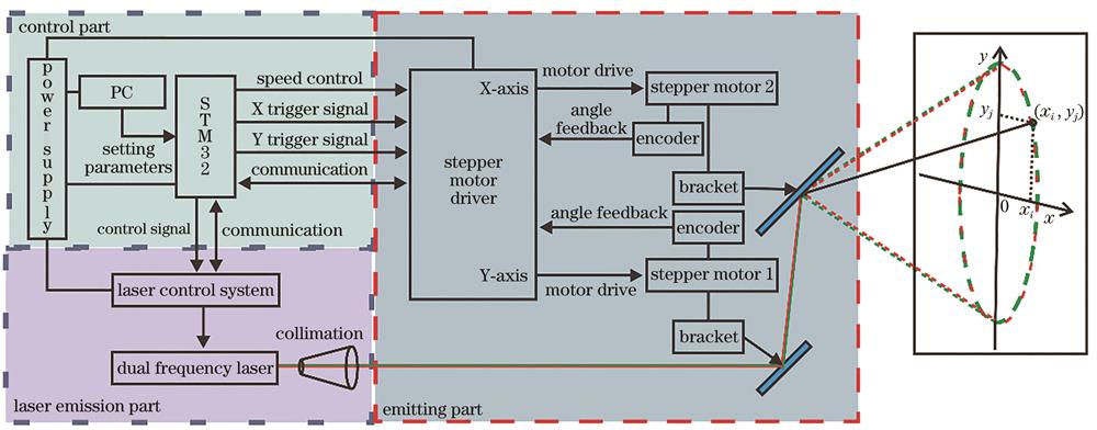
    Fig. 1. General block diagram of two-dimensional galvanometer scanning system
    Scanning diagram. (a) y-axis swing; (b) x-axis swing
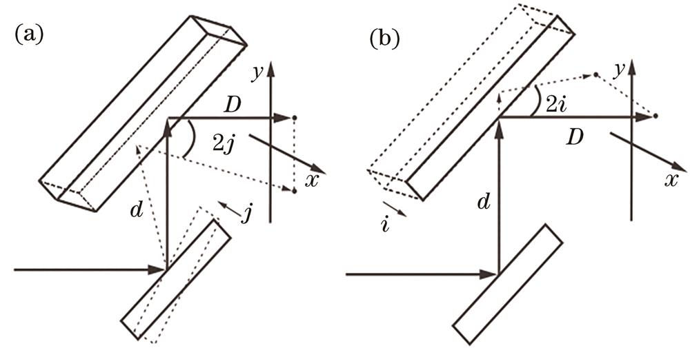
    Fig. 2. Scanning diagram. (a) y-axis swing; (b) x-axis swing
    Comparison of algorithm output values before and after improvement. (a) x coordinate values comparison; (b) y coordinate values comparison; (c) Δx coordinate values comparison; (d) Δy coordinate values comparison
    Fig. 3. Comparison of algorithm output values before and after improvement. (a) x coordinate values comparison; (b) y coordinate values comparison; (c) Δx coordinate values comparison; (d) Δy coordinate values comparison
    Control experiment
    Fig. 4. Control experiment
    Two-dimensional galvanometer scanning experiment. (a) Two-dimensional galvanometer scanning; (b) 20° cone scanning trajectory
    Fig. 5. Two-dimensional galvanometer scanning experiment. (a) Two-dimensional galvanometer scanning; (b) 20° cone scanning trajectory
    Scanning trajectory's simulation. (a) 10° scanning trajectory; (b) 20° scanning trajectory; (c) 20° scanning trajectory; (d) 60° scanning trajectory
    Fig. 6. Scanning trajectory's simulation. (a) 10° scanning trajectory; (b) 20° scanning trajectory; (c) 20° scanning trajectory; (d) 60° scanning trajectory
    20° conical scanning trajectory and optical system transverse angle error after compensation. (a) Scanning trajectory of 20° cone after compensation; (b) comparison of lateral angle errors before and after compensation
    Fig. 7. 20° conical scanning trajectory and optical system transverse angle error after compensation. (a) Scanning trajectory of 20° cone after compensation; (b) comparison of lateral angle errors before and after compensation
    IconScanning angle /(°)Motor speed /rpsFlight speed /(km·h-1Scanning width /mLaser feet density /(spots·m-2
    a101.4200175.01.30
    b201.1200352.71.00
    c206.0200352.75.59
    d606.02001154.71.33
    Table 1. Values of simulate variable scanning trajectory
    Gouqing Zhou, Gangchao Lin, Xiang Zhou, Yizhi Tan, Weihao Li, Xianxing Li, Ronghua Deng. Controlling Scanning Trajectory of Two-dimensional Galvanometer Based on Bresenham Algorithm[J]. Laser & Optoelectronics Progress, 2021, 58(23): 2312001
    Download Citation