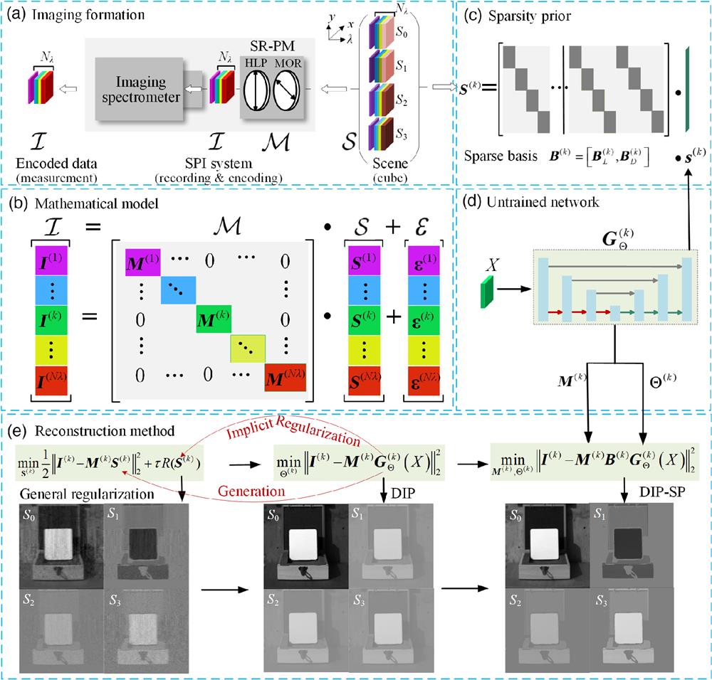
Fig. 1. Schematic of the SPI framework with the passive SR-PM scheme. (a) Imaging formation by integrating the SR-PM with general spectrometer. (b) Forward mathematical model with different colors indicating different spectral bands. (c) Combined sparse representations in transform domain to achieve faster convergence. (d) Untrained network acts as implicit regularization and generator. (e) The reconstruction method is transferred from the CS method with apparent regularization and manual fine-tuning to the unconstrained DIP that uses an untrained network without manual tuning regularization, then to the DIP-SP with the sparse representation constraint and self-calibration ability, which achieves the best performance.

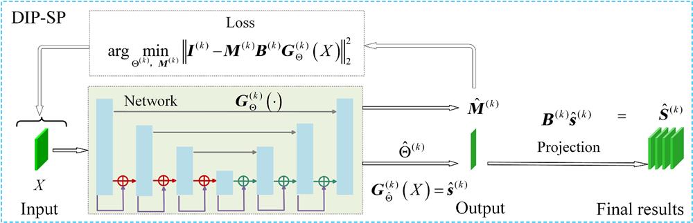
Fig. 2. Processing pipeline of the proposed DIP-SP method.

Fig. 3. Simulated results for the reconstructed images of full-Stokes parameters ($S_0$, $S_1$, $S_2$, and $S_3$) at the spectral band of 550 nm from different algorithms: TwIST-TV, TwIST-SP, DIP, and DIP-SP under the two noise levels ($\sigma =0.05$ and $\sigma =0.2$). Average PSNR and SSIM relative to the GT over all 100 spectral bands are presented just below each image.

Fig. 4. Simulated results (TwIST-TV, green dashed-dotted line; TwIST-SP, blue dashed line; DIP, purple dotted line; DIP-SP, red star-marked dotted line; GT: black solid line) for the average spectropolarimetric curves and error curves over a homogeneous area of $5\text{pixels}\times 5\text{pixels}$. The Stokes parameters ($S_0$, $S_1/S_0$, $S_2/S_0$, and $S_3/S_0$) are in the left column and derived angle of polarization (AOP), degree of linear polarization (DOLP), degree of circular polarization (DOCP), degree of polarization (DOP) in the right column, respectively.

Fig. 5. Simulated results for the reconstructed images of full-Stokes parameters ($S_0$, ${\mathit{S}}_1$, $S_2$, and $S_3$) over the spectral bands of 450, 550, and 650 nm from the TwIST-SP to DIP-SP methods, respectively. The PSNRs and SSIMs relative to the GT at each spectral band are provided below each image. (a) Low-noise level ($\sigma =0.05$) and (b) high-noise level ($\sigma =0.2$).

Fig. 6. Scheme of our miniature snapshot ORRISp. (a) Optical scheme and (b) prototype. MOR, multiple-order retarder; HLP, horizontally linear polarizer; AA, aperture array; LA, lenslet array; BA, baffle array; CVF, continuous variable filter; and FPA, focal plane array.

Fig. 7. Lab scene experiment. Experimental setting (top left) and the color-checker covered with different polarizers as test scene (top right). (a) The red-square mark area is the linear polarizer; (b) the yellow-square mark area is the left-circular polarizer; and (c) the azure-square mark area is the linear polarizer. Lower parts are reconstructed Stokes parameters ($S_0$, $S_1$, $S_2$, and $S_3$) at 550 nm from the TwIST-SP and DIP-SP methods at two exposure time of 60 and 150 ms, respectively.

Fig. 8. Lab experimental spectropolarimetric curves ($S_0$, $S_1/S_0$, $S_2/S_0$, and $S_3/S_0$) of the three selected areas that are shown in the top right of Fig. 7. (a) Red-square mark area; (b) yellow-square mark area; and (c) azure-square mark area.

Fig. 9. Outdoor scene experiment. The reconstructed results at the exposure time of 50 ms for the CIE color fusion image $S_0$ and the gray images ($S_1/S_0$, $S_2/S_0$, and $S_3/S_0$) over the four spectral bands of 480, 550, 600, and 700 nm, respectively. The images from the polarization camera at 550 nm are used for the GT. The spectropolarimetric curves ($S_0$, $S_1/S_0$, $S_2/S_0$, and $S_3/S_0$) of the selected point on the vehicle sunroof are plotted, where only the spectrum $S_0$ has the GT from the fiber spectrometer.

Fig. 10. Dependence of reconstruction quality individually on the fast-axis orientation $\theta$ and the thickness $d$ of the MOR in the SR-PM scheme using the DIP-SP method.

Fig. 11. (a) and (b) The tolerances of the initialization values $(d_i,{\theta }_i)$ from the practical values $(d_p,{\theta }_p)$ of retarder, respectively, under different noise levels.

Fig. 12. History of PSNR and SSIM values of the reconstruction results by the overparameterized network (Res-Unet) and underparameterized network (deep decoder) with respect to the iterations. The inset represents the $S_0$ image every 500 iterations (the upper and lower rows are from the underparameterized and overparameterized network, respectively).

Fig. 13. Acceleration strategy of the DIP-SP processing the images of all spectral bands one by one.

Table 1. The average absolute errors and RMSEs of spectropolarimetric curves (TwIST-TV, TwIST-SP, DIP, and DIP-SP) relative to the GT.

Table 2. Lab experimental results for the RMSEs of reconstructed spectropolarimetric curves relative to the results from the DIP-SP method at the long exposure time of 150 ms.

Table 3. Outdoor experimental results for the average PSNRs and SSIMs at 550 nm of each method.

Table 4. Iteration statistics for the simulated and experimental data using the speed-up DIP-SP.