Compressive full-Stokes spectropolarimetric imaging (SPI), integrating passive polarization modulator (PM) into general imaging spectrometer, is powerful enough to capture high-dimensional information via incomplete measurement; a reconstruction algorithm is needed to recover 3D data cube (x, y, and λ) for each Stokes parameter. However, existing PMs usually consist of complex elements and enslave to accurate polarization calibration, current algorithms suffer from poor imaging quality and are subject to noise perturbation. In this work, we present a single multiple-order retarder followed a polarizer to implement passive spectropolarimetric modulation. After building a unified forward imaging model for SPI, we propose a deep image prior plus sparsity prior algorithm for high-quality reconstruction. The method based on untrained network does not need training data or accurate polarization calibration and can simultaneously reconstruct the 3D data cube and achieve self-calibration. Furthermore, we integrate the simplest PM into our miniature snapshot imaging spectrometer to form a single-shot SPI prototype. Both simulations and experiments verify the feasibility and outperformance of our SPI scheme. It provides a paradigm that allows general spectral imaging systems to become passive full-Stokes SPI systems by integrating the simplest PM without changing their intrinsic mechanism.
High-dimensional optical information, such as irradiance, spectrum, space, polarization, and phase, are vital for comprehensively noninvasive characterization of targets over diverse scenes.1,2 The acquisition of maximal information using a single integrating system is highly desirable in consideration of volume, weight, integration, portability, and cost.3–8 As shown in Fig. 1, spectropolarimetric imaging (SPI), which integrates a polarization modulator (PM) into an imaging spectrometer, is a kind of such a versatile integrating system,5,9–15 which can obtain a spatiospectrally resolved 3D data cube (, , and ) for each of interested Stokes parameters (, , , and ). It has aroused wide applications in the fields of aerosol detection,16 planetary exploration,17 remote sensing,18 biomedical diagnosis,19,20 etc. The design chain of SPI system involves three aspects: the PM, the imaging spectrometer, and a reconstruction algorithm. It is extremely meaningful to design a kind of advanced PM and algorithm that can directly adapt to general imaging spectrometers (multispectral/hyperspectral systems), including scanning (whisk broom, push broom, windowing, and framing)21 and snapshot modes.6,7
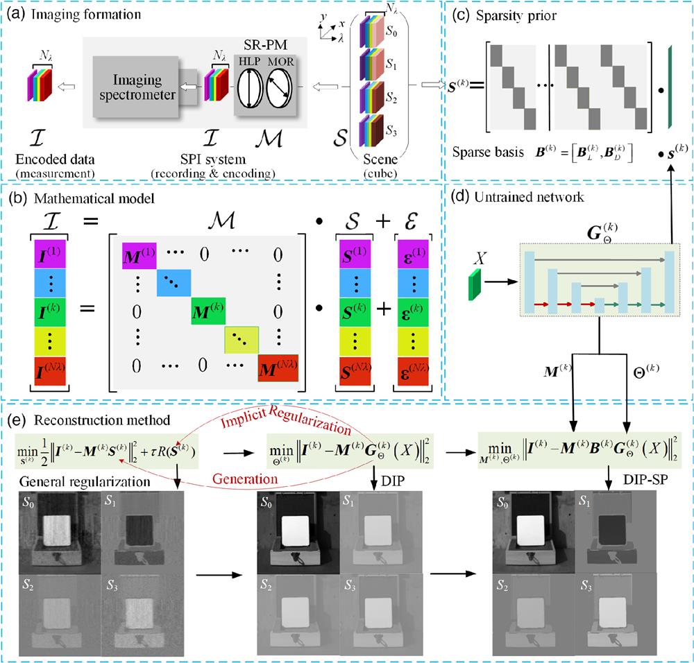
Figure 1.Schematic of the SPI framework with the passive SR-PM scheme. (a) Imaging formation by integrating the SR-PM with general spectrometer. (b) Forward mathematical model with different colors indicating different spectral bands. (c) Combined sparse representations in transform domain to achieve faster convergence. (d) Untrained network acts as implicit regularization and generator. (e) The reconstruction method is transferred from the CS method with apparent regularization and manual fine-tuning to the unconstrained DIP that uses an untrained network without manual tuning regularization, then to the DIP-SP with the sparse representation constraint and self-calibration ability, which achieves the best performance.
The PM is a key component that determines the number of measurements in the polarization dimensionality. According to the sampling mechanism, the PMs can be classified into two types5,7: a well-sampled PM and an undersampled PM. For the former, the number of polarization measurements is equal to the number of interested Stokes parameters. In this case, time-sequence active scanning hardware in a single optical path or snapshot passive hardware using multiple parallel optical paths are usually employed.5 As a result, the acquisition, storage, and processing of these measurements may result in significant time costs, power consumption, space/memory footprint, and possible human resource costs. Meanwhile, designing and building such hardware is expensive and complex.7 For the latter, the number of measurements is less than the number of interested Stokes parameters. In this case, part of the burden from hardware is shifted to a postprocessing algorithm by designing the active or passive undersampled PMs and jointly developing corresponding reconstruction algorithms. As a result, the SPI based on the undersampled PM becomes a kind of computational imaging mechanism that includes a hardware encoder plus a software decoder.
As a typical passive undersampled PM scheme, double multiple-order retarders (MORs) followed a polarizer (termed DR-PM) along a single optical path have the advantages of passive modulation, compact structure, and freedom design space, which have led to many SPI system designs based on existing general imaging spectrometers.9–15 Initially, the Fourier transform method (FTM) based on an analytically physical model was developed and then frequently used to extract polarization channels in the Fourier domain of modulated spectra.10 Although the FTM is a straightforward method, it has some drawbacks, such as channel cross talk, band-limited high-frequency loss, sensitivity to noise, and needing accurate polarization calibration.22–26 Later, optimization-based algorithms, such as compressive sensing (CS) with prior knowledge, have been proposed to overcome the above issues.27,28 While the high-frequency loss and noise sensitivity have been alleviated, accurate polarization calibration with extra precise elements/setups is still needed. The rigorous design of an SPI system is thus transferred to the polarization calibration system, which is a change in form but not in content. Meanwhile, we have developed a continuous sliding iterative method (CSIM) without the need for polarization calibration,29,30 which can converge well by just letting the initialization be of nominal value. The spectropolarimetric resolution recovered from the CS and CSIM retains the intrinsic spectral resolution of the imaging spectrometer used. This point is very important for the imaging spectrometers that only have modest spectral resolution.12,19,31,32 However, the FTM, CS, and CSIM methods are still subject to noise perturbation, since the SPI systems usually have lower flux due to a narrow spectral band and the use of a polarizer. In addition, the FTM and CS methods are enslaved to systematic errors originating from double MORs. Therefore, much labor is spent on the compensation and calibration of the systematic errors such as phase shift, azimuthal misalignment, and temperature effects.22–26 Recently, data-driven deep-learning-based techniques have been proposed to enhance reconstruction quality.33–35 However, the collection of a large amount of labeled data for kinds of application scenes is challenging. Further, the training data and trained networks are usually system-specific, which is difficult to be extended to other SPI systems. Conversely, model-driven reconstruction methods are still expected to label the data for feeding such data-driven deep-learning-based approaches.
Sign up for Advanced Photonics Nexus TOC. Get the latest issue of Advanced Photonics Nexus delivered right to you!Sign up now
To avoid the above dilemma, it is important to determine whether it is feasible to construct the simplest undersampled full-Stokes PM just using a single MOR followed a polarizer (termed SR-PM) along a single optical path and build novel model-driven method to reconstruct a spatiospectrally resolved 3D cube for each of four Stokes parameters (, , , and ) from incomplete measurement. Although such an SR-PM scheme definitely has the advantages of volume, alignment, assembly, and cost compared to the DR-PM scheme, the reconstruction algorithm crisis would be aggravated in the absence of clarity. Recently, state-of-the-art deep-image prior (DIP) methods using untrained networks have been proposed for image denoise and restoration with provable convergence.36–47 Therein, the structure of an untrained network with randomly initialized weights can function as a prior on image statistics without any training, mainly because deep neural networks are good at representing and generating realistic images.48–50 Specifically, an untrained network is paired with a physically differentiable forward-imaging model in which the network weights are updated through a loss function comparing the experimental measurement and the generated measurement from the network output passed through the forward imaging model. Therefore, the DIP method is expected to be promising to solve the reconstruction issues of the SPI. However, preliminary applications of the DIP methods on other computational imaging problems38–47, would not account for practical issues in the SPI systems. It was found that if we directly use the DIP method to solve the inverse problem of the SPI, the inversion results tend to be trapped in a pseudo-solution, where all generated images show the similar still detail, but modulated with constants (see Secs. 4 and 5), mainly because the problem in the SPI is more challenging owing to its high dimensionality. This kind of challenge is our motivation to further constrain the DIP by incorporating proper prior knowledge about optical physics in systems or scenes. That is, the physical imaging models of the SPI should be built reasonably, and further regularization should be introduced for the inverse problem. Hereby, we devise a DIP plus sparsity prior (DIP-SP) method to make the encoding and decoding of the SR-PM scheme become feasible and more efficient. Meanwhile, self-calibration is achieved with the algorithm itself; then accurate polarization calibration is not necessary.
Toward the above-mentioned ends, the novelty of this paper through the encoding hardware to decoding software is threefold: (1) The principle and forward-imaging model of SPI based on the SR-PM is presented. (2) By incorporating SP into the SPI forward model, a physically constrained DIP-SP method based on an untrained network is developed. In particular, the method does not need any training data and accurate polarization calibration and can simultaneously reconstruct the 3D data cube of each Stokes parameter and achieve the self-calibration of measurement matrix. (3) As an instance, we integrate the SR-PM in front of our miniature snapshot imaging spectrometer to form a single-shot SPI prototype. Both simulation and experimental results show that the proposed DIP-SP algorithms make the SR-PM feasible and more robust to noisy perturbation. The rest of paper is organized as follows. Section 2 presents the SPI forward model. The proposed DIP-SP method is presented in Sec. 3. Extensive simulations and real-world experiments using our miniature SPI prototype are provided in Sec. 4. Section 5 provides a discussion and Sec. 6 provides the conclusion.
2 SPI Forward Model
As shown in Fig. 1(a), a full-Stokes SPI system is built by integrating the SR-PM into a general imaging spectrometer.5–7,21 Herein, the SR-PM consists of a fixed MOR following a horizontally linear polarizer (HLP), which is the simplest undersampled full-Stokes PM. The sampling mechanism of the SPI mainly consists of two steps. First, the spatiospectrally distributed 3D data cube (, , and ) for each of four Stokes parameters (, , , and ) are compressively encoded by the SR-PM. Second, the encoded spectropolarimetric data cube is then recorded by the imaging spectrometer used. The working mode of the imaging spectrometer can be whisk broom, push broom, windowing, framing, or snapshot. Either way, the encoded spectropolarimetric data cube should be output for subsequent reconstruction.
Mathematically, a 2D scene can be characterized by a spatiospectrally distributed 3D data cube (, , and ) for each of the Stokes parameters (, , , and ), as shown in the right part of Fig. 1(a). The data cube slices of the ’th spectral band are expressed as , where , , , and denote the scene height, scene width, the number of spectral bands, and the number of interested Stokes parameters (herein ), respectively. It is first compressively modulated by the SR-PM with measurement matrix ; then the encoded spectropolarimetric slice is recorded by the imaging spectrometer as where indicates noise; and denote the ’th measurement matrix () and corresponding 2D distribution of Stokes parameter, respectively; and represents the Hadamard (element-wise) product.
As shown in Fig. 1(b), the forward model of SPI at the ’th spectral band can be linearly expressed as where and with vectorizing the 2D matrix by lexicographically stacking columns. Correspondingly, the vectorization of the whole Stokes parameters is where indicates transpose operation. The measurement matrix is a concatenation of diagonal matrices, where the constant coefficient 1/2 means the flux is halved due to the use of a polarizer. The slice of each spectral band is characterized by similar expressions. Correspondingly, the measurement of all spectral bands is obtained by integrating all slices, where
As can be seen, the modulation mechanism of SR-PM is characterized by the measurement matrix , which can be derived using Muller–Stokes calculus as (Note 1 in the Supplementary Material) where and are the maximum and minimum transmittance that account for the imperfection of the polarizer; ; is the thickness, is the ’th wavelength; and and are the extraordinary and ordinary refractive indices of the MOR, respectively. It is observed that the number and complexity of effective arguments depend on the two free parameters . If we set to simplify the arguments, only partial Stokes parameters could be modulated. In addition, if we let the MOR be an achromatic waveplate for simplification, the system spectral range would be narrowed and unnecessary cost would be induced. To simultaneously modulate all Stokes parameters (, , , and ) with generality, we should let and regardless of the phase retardance , although the arguments would be not so clear and simple. The effects of free parameters on the reconstruction quality will be explored in Sec. 5 for the optimal measurement matrix and its tolerance. For the DR-PM scheme,9–15 we also can derive the corresponding measurement matrix, and the following methods also adapt to its modulation.
3 Reconstruction Methods
For the inverse problem of SPI, the measurement does not resemble the reconstructed image; instead, the scene is related to the measurement through the forward-imaging model that describes the physics of the image formation problem. To reconstruct Stokes parameters at different wavelengths from Eq. (5), one may use the pseudo-inverse of measurement matrix as a fast method. However, it should be noted that the forward-imaging model in Eqs. (2) or (5) is ill-posed, since the number of unknowns is times that of knowns in the measurement. This means that the measurement is incomplete, and computational reconstruction is needed. As a matter of convenience, it is recommended to independently reconstruct the Stokes parameters at each wavelength. We formulate the inverse problem by creating the mathematical model with an inspiration from the CS. The inverse problem aims to recover the image slices of the four Stokes parameters from the encoded spectropolarimetric slice via proper regularization, where is the data-fidelity term and is the regularization term with a tuning parameter . To obtain the 3D data cube of each Stokes parameter with high quality, generally the measurement matrix should be calibrated accurately. However, it is hard to solve Eq. (8) directly, even using state-of-the-art solvers [e.g., the gradient projection for sparse reconstruction (GPSR)51 or the two-step iterative shrinkage/thresholding algorithm (TwIST)]52 with elaborately handcrafted regularization such as the sparsity or total variation (TV). Its noise robustness and reconstruction quality are subject to handcrafted regularizations or scene types, as shown in Fig. 1(e). In addition, it is necessary that the measurement matrix be definitely known using accurate polarization calibration. Thus, it is desirable to develop an advanced algorithm with powerful regularization but without manual tuning of parameters, meanwhile incorporating self-calibration of the measurement matrix into the algorithm.
3.1 DIP Plus SP Method
The state-of-the-art DIP via untrained network has been proposed for the inverse problem of computational imaging with provable convergence36,37 and shown to be particularly effective for many applications.38–47 In the following sections, we use DIP to solve the SPI inverse problem. As shown in Fig. 1(d), assuming the mapping function of the untrained network is specified by a set of parameters , the inverse problem in Eq. (8) is then replaced as where indicates the input of the untrained network. It is interesting to note that the function of regularization term in Eq. (8) is replaced by the implicit DIP captured by the untrained network in the data-fidelity term. With the known measurement matrix , the iterative optimization of Eq. (9) is to find a set of optimal parameters of the untrained network that map the input to the desired signal as
As can be seen, the main advantage of the DIP method is that the input is just the without any need of the ground truth (GT) . However, we found that it is also hard to optimize such preliminary DIP method in Eq. (9) with satisfactory results. The inversion results tend to be trapped in a pseudo-solution, where all generated images show similar detail, but modulated with constants (see Sec. 4.2 and Sec. 5), mainly because the SPI is higher-dimensional and more ill-posed compared to previous applications.38–47 In addition, the measurement matrix in Eq. (9) also needs to be definitely determined before the reconstruction process. These kinds of challenges are our motivation to further constrain the DIP by introducing reasonable regularization.
Since the SP has been shown to be more effective on computational imaging problems,53 it is reasonable to incorporate the SP into the DIP for solving the SPI problem, forming the DIP-SP method. Therefore, as shown in Fig. 1(c), we make a prior assumption that the Stokes parameters of the 2D scene can be sparsely represented on suitable bases as where denote the bases coefficients and is the number of bases coefficients. The bases can be obtained from some transform domains (e.g., undecimated wavelet transform, discrete Fourier transform, discrete Hartley transform, discrete cosine transform, Legendre polynomials) or dictionary learning. In this work, we select the bases from the combined domains, including discrete cosine transform and Legendre polynomials, to maximize earnings of the SP constraint (Note 2 in the Supplementary Material). The Legendre polynomials are an orthogonal basis that are useful to model signals such as linear, quadratic, and cubic polynomials. Further, their scale is small relative to other bases, therefore increasing the speed of calculation. The discrete cosine transform coefficients are helpful in capturing sinusoidal variations. The bases coefficients are from the combination of two bases . The number of total bases coefficients is the summation of the Legendre polynomials coefficients and the discrete cosine transform coefficients .
Then, as shown in Fig. 2, we incorporate the SP constraint in Eq. (11) into the unconstrained DIP optimization in Eq. (9) as
Figure 2.Processing pipeline of the proposed DIP-SP method.
As a result, the prior captured by the untrained network is enhanced due to the additional SP constraint, making convergence easier. In addition, it should be pointed out that we let the network parameters and measurement matrix be optimized simultaneously. Therefore, it is not necessary to explicitly know the measurement matrix , depending on the accurate polarization calibration. Only a warm initialization of is needed for convergence and self-calibration (see discussion in Sec. 5). The optimized mapping function is now used to estimate the bases coefficients ,
The final Stokes parameters are derived using Eq. (10). The input can be random input with similar dimension36–38 or the practical measurement .40,41 If the texture features of the measured spectropolarimetric image resemble the reconstructed images, it is helpful to directly use the practical measurement as the input to speed up convergence.39 By allowing other spectral bands undergo a similar optimization process, the whole Stokes parameters at each spectral band can be inversed one by one. Since the DIP-SP method processes all spectral bands individually, it can be applied to monochromatic, multispectral, and hyperspectral SPI schemes.
3.2 Neural Network Framework and Auto-stopping Criterion
For the DIP method, different kinds of neural networks can be employed.36,37 When the DIP method was debuted, Ulyanvov et al.36 used an overparameterized autoencoder network (i.e., a network with more weights than the number of unknowns). Other preliminary applications also inherit similar overparameterized networks.39–47 However, it is observed that the iteration process cannot stop automatically, since loss function does not monotonously decrease with the iterations. The iteration must be manually stopped in time when the loss begins to increase. It is critical to stop the iteration at a reasonable convergence point in a timely manner. To avoid early stopping or any other further regularization, an underparameterized network, deep decoder, was proposed by Heckel and Hand,38 due to its resemblance to the decoder part of the autoencoder. The deep decoder does not involve convolutions, and has a concise structure that makes itself an image model with a lower-dimensional description. Since the underparameterized network provides a barrier to overfitting, it can enhance the regularization of inverse problems. However, its representation ability on high-dimensional images with complex details lacks evidence.
To ensure the feasibility of our methods, we elect to use the overparameterized network for performance verification (see discussion in Sec. 5). Specifically, a combination of Unet54 and ResNet,55 termed as modified Res-Unet56 (Note 3 in the Supplementary Material), is employed, as shown in Fig. 2(b). While the Unet is a neat end-to-end convolutional neural network for multiscale feature extraction from input images,54 the Res-Net with skip connection can avoid overfitting.55 Therefore, to prevent the over-parameterized Res-Unet from auto-stopping at an early stage, an autostopping criterion (further regularization) must be built. Since the SPI reconstruction is to obtain the spectral images of Stokes parameters, the structural similarity (SSIM) and peak signal-to-noise ratio (PSNR) are two necessary metrics to evaluate the reconstruction quality. Therefore, we build the autostopping criterion by combining the SSIM and PSNR as follows: where is the number of iterations, is the interval of adjacent iterations for average, and and are two small values for stopping. We let the iteration process stop when both Eqs. (15a) and (15b) are satisfied simultaneously. As the criterion considers the average SSIM and PSNR through a series of adjacent iterations, it can avoid the unstable alarm from seldom-rising loss points that cannot easily be distinguished by manual intervention.
4 Implementations and Results
4.1 Competitive Algorithms and Evaluation Metrics
In this section, the performance of the proposed DIP-SP in Eq. (13) is verified by extensive simulations and experiments. In addition, the unconstrained DIP method is also executed for comparison. These DIP methods are implemented with Python version 3.6.13 on the PyTorch 1.9.0 platform. The adaptive moment estimation (Adam) optimizer with a learning rate of 0.01 is used to iteratively update the weights and biases. For comparison, we also implement the CS methods in Eq. (8) with TV regularization and with the same SP, respectively. The TwIST49 is selected as the solver. For convenience, we term these two algorithms as the TwIST-TV and TwIST-SP, respectively. It is found that, for achieving the best results, the regularization parameter should be manually tuned to and the number of iterations in the minimization step in each TwIST iteration be set at 4. All implementations use a machine equipped with AMD Ryzen 7 3700X 8-Core CPU with 16 GB RAM and NVIDIA GeForce GT 1030 GPU.
Two widely quantitative image quality assessment metrics, the PSNR and SSIM, are used to compare the performance. Both of them are spatial measurements, and the higher values indicate spatial reconstruction is good. In addition, the reconstructed spectropolarimetric curves of selected areas are provided for qualitative evaluation. The root mean square error (RMSE) between the GT and the reconstructed curve is used to globally measure the reconstruction quality. The lower the RMSE value, the less the distortion of the reconstructed curve.
4.2 Simulations
4.2.1 Simulation setting
To determine whether the DIP-SP adapts to a scene that has spectropolarimetric curves with different vibration frequencies, we select hyperspectral images from the public data set ICVL57 to manually feed polarization information with different vibration frequencies. The original hyperspectral images in the ICVL have the spatial size of with 361 spectral bands from 400 to 850 nm at a step of 1.25 nm. To generate the controllable polarized spectra with different vibration frequencies, we simply use cosine and sine functions to modulate the spectra . To reduce computation, we crop out the middle part with the spatial size of that include different objects as the test scene, and just extract 100 spectral bands at a step of 4.5 nm for simulations.
The measurement of the encoded spectropolarimetric data cube is generated following the forward-imaging model in Eq. (2). We let the thickness be and the fast-axis orientation be (optimal selections are discussed in Sec. 4.1). Then the practical value of measurement matrix is derived from Eq. (4). For the TwIST-TV, TwIST-SP, and the unconstrained DIP methods, the practical value is necessary and used for reconstruction. However, for the proposed DIP-SP method, the measurement matrix is the optimization objective, as described in Eq. (13). To validate the robustness of DIP-SP, we, by design, let the initialization of DIP-SP method have a random deviation of a maximum of 3% from the practical value (its tolerance is discussed in Sec. 5). In addition, to mimic practical measurements as much as possible, the additive Gaussian noise of zero mean with low and high standard deviations of and , respectively, are added to the normalized measurements for comparison.
4.2.2 Simulation results
Figure 3 shows the reconstructed images of Stokes parameters (, , , and ) at the spectral band of 550 nm under the two noise levels ( and ), respectively. It can be seen that for CS methods, while the TwIST-TV performs the worst, the TwIST-SP is sensitive to noise perturbation. For the DIP methods, the unconstrained DIP method is totally invalid. In contrast, the DIP-SP method achieves the best results at any noise level. For the intensity image , the PSNRs of TwIST-SP and DIP-SP decrease about 6.35 and 5.11 dB, and the SSIM decreases about 0.052 and 0.051, respectively, from the low-noise level () to the high-noise level (). For all the polarization images (, , and ), the PSNRs decrease about 5.5 dB and 4.8 dB, and the SSIM decreases about 0.046 and 0.044, respectively. However, the DIP-SP method still achieves high-quality reconstruction at the high-noise level.
Figure 3.Simulated results for the reconstructed images of full-Stokes parameters (, , , and ) at the spectral band of 550 nm from different algorithms: TwIST-TV, TwIST-SP, DIP, and DIP-SP under the two noise levels ( and ). Average PSNR and SSIM relative to the GT over all 100 spectral bands are presented just below each image.
Figure 4 shows the reconstructed average spectral curves of all polarization parameters over a homogeneous area of ; their average absolute errors and RMSEs relative to the GT are listed in Table 1. It is found that both the TwIST-TV and the unconstrained DIP methods are almost invalid at any noise level. Even though the spectropolarimetric curves of TwIST-SP approximate to the GT just at the low-noise level (), they have obvious spectral distortions. Although both the TwIST-SP and DIP-SP methods degrade with the increase of noise, the results of DIP-SP method still conform well to the GT. When the initialization is equal to the practical value of the measurement matrix, the average absolute errors of the reconstructed Stokes parameters from the DIP-SP are at the low-noise level () and at the high-noise level (). If the initialization has the random deviation of a maximum of 3%, the average error of reconstruction is less than 0.01, still within the tolerance range, as shown in Table 1. In summary, the DIP-SP method is most robust to the noise perturbation and spectral vibration attribute to the use of the SP constraint as well as the self-calibration of measurement matrix . More detailed analyses about the influence of the spatial resolution and spectral resolution on the DIP-SP reconstruction are presented in Note 4 in the Supplementary Material.
Figure 4.Simulated results (TwIST-TV, green dashed-dotted line; TwIST-SP, blue dashed line; DIP, purple dotted line; DIP-SP, red star-marked dotted line; GT: black solid line) for the average spectropolarimetric curves and error curves over a homogeneous area of . The Stokes parameters (, , , and ) are in the left column and derived angle of polarization (AOP), degree of linear polarization (DOLP), degree of circular polarization (DOCP), degree of polarization (DOP) in the right column, respectively.
Figure 5(a) shows the reconstructed images of Stokes parameters (, , , and ) just using TwIST-SP and DIP-SP methods over the spectral bands of 450, 550, and 650 nm, respectively, at the low-noise level (). As can be seen, the results of DIP-SP preserve more features across the spectral bands, and the results of TwIST-SP have obvious artifacts. The average PSNRs and SSIMs of DIP-SP in each band are higher than those of the TwIST-SP, respectively, by 9.9 dB and 0.078 for the images, and by 10.52 dB and 0.073 for (, , and ) images.
Figure 5.Simulated results for the reconstructed images of full-Stokes parameters (, , , and ) over the spectral bands of 450, 550, and 650 nm from the TwIST-SP to DIP-SP methods, respectively. The PSNRs and SSIMs relative to the GT at each spectral band are provided below each image. (a) Low-noise level () and (b) high-noise level ().
Similarly, Fig. 5(b) shows the reconstructed images of Stokes parameters (, , , and ) at the high-noise level (). The images of TwIST-SP exhibit evident artifacts, especially on the white wall. In contrast, the images of DIP-SP retain clearer details and have the best quality. The PSNR and SSIM of DIP-SP are better than those of the TwIST-SP by 10.95 dB and 0.092 for the images and by 10.52 dB and 0.091 for (, , and ) images.
4.3 Experiments
4.3.1 Miniature optically replicating and remapping imaging spectropolarimeter
In this work, we let the imaging spectrometer in Fig. 1(a) be our snapshot ORRIS,58 then the SPI system become a snapshot optically replicating and remapping imaging spectropolarimeter (ORRISp).59 The passive SR-PM is used to encode the spectropolarimetric images. The ORRIS is used to obtain the spectropolarimetric images encoded by the SR-PM. However, our pioneer prototypes of ORRIS58 and ORRISp59 are lengthy due to the cascaded imaging objective lens (OL), field stop, and collimating lens. These optical elements are mainly used to prevent adjacent subimages of lenslet array (LA) from overlapping. Actually, the size of the subimage can be controlled by inserting a baffle array (BA) between the LA and the focal plane continuous variable filter (CVF), as shown in Fig. 6(a). In this case, the fore optic is removed for miniaturization and then the optical flux is improved, largely due to the reduction of multiple reflection surfaces. In addition, the previous DR-PM with the double MORs is now replaced by the SR-PM with the single MOR for further simplification and easy alignment and assembly. Finally, a miniature ORRISp is developed, which is termed as MINI-ORRISp. Its detailed design, calibration, and testing can be found in reference.60 Correspondingly, the working spectral range is extended from 450 to 750 nm for the pioneer ORRISp to 400 to 850 nm for the MINI-ORRISp due to the remove of achromatic quarter-wave plate. More important, the spatiospectrally resolved 3D data cube (, , and ) of full Stokes parameters (, , , and ) can be simultaneously obtained by the MINI-ORRISp prototype, relative to the pioneer ORRISp prototype that just focused on the linear Stokes parameters (, , and ).
Figure 6.Scheme of our miniature snapshot ORRISp. (a) Optical scheme and (b) prototype. MOR, multiple-order retarder; HLP, horizontally linear polarizer; AA, aperture array; LA, lenslet array; BA, baffle array; CVF, continuous variable filter; and FPA, focal plane array.
Figure 6(b) shows the final prototype of MINI-ORRISp. The MOR is made from quartz, with a thickness of . The HLP is an ultrabroadband wire grid polarizer. They are assembled in the same anodized aluminum lens tube. The LA is array with a pitch of 3 mm and a focal length of 9 mm. The row direction of the LA has an inclination angle of 6.34° relative to the CVF’s wave band. The size of the CVF is . The center wavelength varies along the 25 mm side in the global axis. The FPA is a CCD array with the spatial resolution of and the pixel size of . The volume of MINI-ORRISp prototype is largely miniaturized to 80 mm (length) × 70 mm (width) × 70 mm (height), and the weight is reduced to 700 g. Within a single exposure time, the MINI-ORRISp can get 81 raw subimages. After registering all subimages to the center one, we can remap out the encoded spectropolarimetric images with the spatial resolution of over spectral bands. The spectral resolution at each spectral band is around 3.5% of the central wavelength. For the LA arrangement, two main considerations come into play. The first one is the trade-off between spatial and spectral resolution. The second is how to maximize the utilization of the CVF and effective CCD area while avoiding complex processing. According to the principle of optical replication and remapping,58 the spectral resolution increases with the number of lenses in each row of the LA, but the spatial resolution ( and ) will decrease due to the limited area of the CCD. Therefore, a reasonable arrangement of the LA must be a compromise between spatial and spectral resolution. Based on the above considerations, the size of the subimage is designed to be 400 () pixels × 400 () pixels, and the LA is designed to be . It should be noted that, to maximize the use of the CVF and CCD, a portion of LA on the marginal area is deliberately designed to be outside the effective imaging area. Specifically, the upper half of the first row of the LA and the lower half of the last row of the LA do not cover the CVF, which means these parts do not participate in the replication of subimages and continuous filtering. Therefore, after remapping, the LA corresponds to spectral bands.
4.3.2 Experimental setting
We first use the MINI-ORRISp to record the encoded spectropolarimetric images of a real-world scene in a single shot and then apply both the TwIST-SP and DIP-SP methods to decode a spatiospectrally resolved 3D data cube of for each of four Stokes parameters (, , , and ), respectively. For the two reconstruction methods, the measurement matrix of system is roughly calibrated using an He–Ne laser and a commercial polarization analyzer (Thorlabs, PAX1000) pointing to several field points of the PM. Other field points and spectral bands are simply interpolated and derived as the initializations. Predictably, the performance of the TwIST-SP method will be degraded further relative to the simulation experiments, in which the practical measurement matrix has been exactly employed for reconstruction. In contrast, the performance of the DIP-SP method will be retained, since the measurement matrix can be self-calibrated during iteration. In addition, a diffuse reflection standard whiteboard is employed as a white reference for each test scene to remove the disturbance of ambient light during acquisition. A monochromatic polarization camera is built and calibrated to obtain the ground truth images of full Stokes parameters. It consists of a high-resolution camera modulated by a rotatable linear polarizer and filtered by a bandpass filter centered at 550 nm with a bandwidth of 10 nm. A standard fiber spectrometer with a fiber probe is used to sample the GT of spectrum for the selected area. An RGB camera is employed to acquire the GT of color images. We let the polarization camera, RGB camera, and fiber spectrometer work with the best settings to get the data as GTs.
4.3.3 Laboratory scene
For the laboratory scene, the experimental setup is shown in the upper left of Fig. 7. A color-checker covered with linear polarizers and circular polarizers of different polarization directions is used as a test scene in the upper right of Fig. 7. The illumination source is a fluorescent lamp. The MINI-ORRISp, the polarization camera, the RGB camera, and the fiber spectrometer observe the color-checker at the same time. The MINI-ORRISp operates at two exposure time of 150 and 60 ms for noisy comparison. For all measurements, the longer the exposure time, the higher the signal to noise ratio (SNR).
Figure 7.Lab scene experiment. Experimental setting (top left) and the color-checker covered with different polarizers as test scene (top right). (a) The red-square mark area is the linear polarizer; (b) the yellow-square mark area is the left-circular polarizer; and (c) the azure-square mark area is the linear polarizer. Lower parts are reconstructed Stokes parameters (, , , and ) at 550 nm from the TwIST-SP and DIP-SP methods at two exposure time of 60 and 150 ms, respectively.
The lower part of Fig. 7 shows the reconstructed Stokes parameter images (, , , and ) at 550 nm with the statistic PSNR and SSIM results for each algorithm. Obviously, the reconstruction quality of two methods at the long exposure time is better than that at the short exposure time. While the DIP-SP method achieves better results, the TwIST-SP method is very sensitive to noise perturbation at any exposure time. This phenomenon is consistent with the simulation results in Sec. 4.2.
Figure 8 plots the average spectropolarimetric curves (, , , and ) of three selected areas (a, b and c with ) that are shown in the upper right of Fig. 8. Only the spectra have the GTs that captured using the fiber spectrometer. Clearly, the DIP-SP is champion for the spectra at each exposure time. In contrast, the TwIST-SP is barely acceptable only after a long exposure time and is futile at the short exposure time. Unsurprisingly, the spectropolarimetric curves (, , and ) are slowly varying, mainly because the selected areas are almost fully polarized by the covered polarizers. We let the spectropolarimetric curves from the DIP-SP at the long exposure time of 150 ms be references; then the RMSEs of other results are calculated in Table 2. Clearly, the performance of TwIST-SP at any exposure time is worse than that of the DIP-SP at the short exposure time.
Figure 8.Lab experimental spectropolarimetric curves (, , , and ) of the three selected areas that are shown in the top right of Fig. 7. (a) Red-square mark area; (b) yellow-square mark area; and (c) azure-square mark area.
Table 2. Lab experimental results for the RMSEs of reconstructed spectropolarimetric curves relative to the results from the DIP-SP method at the long exposure time of 150 ms.
In the laboratory scene, we have verified the performance of our system and algorithms on a fully polarized scene with different exposure time. However, outdoor natural scenes are totally different due to the lack of a high degree of polarization and the fullnes of a complex background. We photographed a car parked on the road on a sunny day, with the exposure time decreased to 50 ms. Figure 9 shows the reconstructed images of Stokes parameters (, , , and ) at 480, 550, 600, and 700 nm, respectively. The PSNR and SSIM relative to the GT captured by the polarization camera at 550 nm are calculated in Table 3.
Figure 9.Outdoor scene experiment. The reconstructed results at the exposure time of 50 ms for the CIE color fusion image and the gray images (, , and ) over the four spectral bands of 480, 550, 600, and 700 nm, respectively. The images from the polarization camera at 550 nm are used for the GT. The spectropolarimetric curves (, , , and ) of the selected point on the vehicle sunroof are plotted, where only the spectrum has the GT from the fiber spectrometer.
As can be seen, for the TwIST-SP method, the details of images (, , and ) are blurry in each narrow spectral band caused by noise. The DIP-SP has the better reconstruction quality in all bands. The spectropolarimetric curves on the vehicle sunroof are plotted. Only the spectra of the DIP-SP are consistent with the GT that is obtained using the fiber spectrometer. The TwIST-SP result suffers from large vibrations and deviations. Since the sunroof has high reflection, the reflected spectra are partially polarized and slowly varying, as indicated by the spectropolarimetric curves (, , and ) from the DIP-SP method. The value of each curve at 550 nm complies with the GT from the polarization camera. Since the circular polarization component of nature scene is very weak, both the hardware and software should have good robustness to noise.
To demonstrate the necessity of our MINI-ORRISp as well as the DIP-SP method over previous methods with rotatable polarizers, the application on real-time acquisition of dynamic scenes is presented in Note 5 and Fig. S4 in the Supplementary Material as well as in Video 1, URL: https://doi.org/10.1117/1.APN.2.3.036009.s1.
5 Discussions
5.1 Optimal Free Parameters
For the SR-PM scheme with the single MOR, the fast-axis orientation and the thickness of the MOR are the two free parameters to encode spectra. The reconstruction quality of the DIP-SP depends on these parameters. Using the simulation data in Sec. 4.2, the PSNR and SSIM as functions of the two parameters, respectively, are plotted in Fig. 10. It is found that the reconstruction quality (PSNR and SSIM) slightly decreases with the increase of and sensitively vibrate with . The optimal values of are 22.5°, 67.5°, 112.5°, and 157.5°. So, we have set in simulations and real-world experiments. We have selected because the reconstruction quality is relatively high and we have a quartz retarder on hand.
Figure 10.Dependence of reconstruction quality individually on the fast-axis orientation and the thickness of the MOR in the SR-PM scheme using the DIP-SP method.
Figure 11 shows the tolerances of the initialization values from the practical values , respectively. That is, for the initialization values within the tolerances, the system can be self-calibrated to the practical value very well. Obviously, the nominal value (, ) is totally embraced in the range of the initialization values. That means we can directly let the nominal values be the warm initialization values under the corresponding noise levels. However, the tolerances are mainly subject to noise perturbation. The tolerances are maximized to (0.053 mm, 15.19°) at (, ) without noise perturbation and they are minimized to (0.04 mm, 5.83°) at (, ) under the highest noise levels. The tolerance on the thickness is tighter and more sensitive to noise than that on the fast-axis orientation, mainly because even a small error on the thickness will incur considerable error on the retardance of the thick retarder. To let the DIP-SP method adapt to general error and noise cases, it is suggested to roughly calibrate the measurement matrix with elementary setup and operation. In our above experimental results, the measurement matrix has been roughly calibrated using an He–Ne laser and a commercial polarization analyzer (Thorlabs, PAX1000) pointing to several field points of the PM. Other field points and spectral bands are simply interpolated and derived as the initializations. In the future, it will be necessary to maximize the tolerance by designing advanced regularization or network and then save the rough calibration procedure.
Figure 11.(a) and (b) The tolerances of the initialization values from the practical values of retarder, respectively, under different noise levels.
5.2 Overparameterized or Underparameterized Networks
The network frameworks may influence the reconstruction performance. In this section, we compare the performance of an overparameterized network (Res-Unet56) and an underparameterized network (deep decoder37) using the simulated scene in Fig. 3. Figure 12 shows the reconstructed PSNR and SSIM of the two networks over the number of iterations, as well as the reconstructed images at 550 nm every 500 iterations. It is found that, without the SP constraint, the reconstruction results of the overparameterized and underparameterized networks tend to be trapped in a pseudo-solution. In this case, as expected, the convergence of overparameterized network first reaches a higher value, then drops to a lower value. Although the convergence of the underparameterized network does not drop in expectation, the reconstructed quality is limited to the lower value. That is, both of them cannot fit the image well. In contrast, with the help of the SP constraint and self-calibration operation, the reconstructed PSNR and SSIM of the two networks can approach the best results. In this case, both the overparameterized and underparameterized networks can converge very well, and there are no overfitting phenomena, even with a large number of iterations. It is interested to found that the under-parameterized network needs more than 3000 iterations to converge, and the restored images become clear at around 3500 iterations. In contrast, the overparameterized network starts to convergence just after 1000 iterations, and the restored images become definite just after 1500 iterations. That is, the over-parameterized network (Res-Unet) converges faster than the under-parameterized network (deep decoder) for our SPI problem, perhaps because the DIP representation ability of the underparameterized network on high-dimensional images is not sufficient.
Figure 12.History of PSNR and SSIM values of the reconstruction results by the overparameterized network (Res-Unet) and underparameterized network (deep decoder) with respect to the iterations. The inset represents the image every 500 iterations (the upper and lower rows are from the underparameterized and overparameterized network, respectively).
For the DIP-SP method, the iterations can be stopped automatically according to the auto-stopping criterion in Eq. (15). As shown in Fig. 12, both the PSNR and SSIM approach to stably smooth values after 1000 iterations for the over-parameterized network with the SP constraint. To let the DIP-SP automatically stop at the optimal iterations of 1500 nearby, we have set the parameters , , and in Eq. (15), respectively. These parameters have been used commonly in simulations and real-world experiments. As a result, the optimization at each spectral band experiences about 3000 iterations for the lab data and around 5800 iterations for the outdoor data in Sec. 4.
5.4 Acceleration Strategy
As shown in Sec. 3.1, the forward-imaging model and inversion are mainly illustrated at the ’th spectral band for simplification. In practice, although we can input the images of all spectral bands simultaneously into the network according to Eq. (5), this would increase the calculation amount and require mass memory. To reduce computation cost, the images can be spatially split into a series of small image patches. But an evident seam would appear by stitching the reconstructed image patches to nonuniform reconstructions.
Hereby, we recommended processing the images of all spectral bands one by one via a similar procedure. As a result, the DIP-SP method reasonably adapts to hyperspectral, multispectral, and monochromatic imaging mechanisms. However, if the iteration time of the first spectral band is , the total time would be (), which is the accumulation of spectral bands. To speed up convergence and reduce iteration time, an acceleration pipeline is proposed in Fig. 13. It is assumed that the images of adjacent bands share similar semantic features. Then, the optimized mapping function for the ()’th band is considered the prior initial mapping function for the ’th band. In addition, it is found that just allowing the last two layers of the optimized network to participate in training for the ’th band is enough to further reduce iterations. The iteration statistics for the simulated and experimental data are listed in Table 4. As can be seen, the first spectral band needs full iterations; subsequent spectral bands just need fewer iterations. As a result, the total iteration time is reduced around 45 times relative to ().
Figure 13.Acceleration strategy of the DIP-SP processing the images of all spectral bands one by one.
However, the total reconstruction time of the DIP-SP method remains a stumbling block for real-time reconstruction, although we have devised the acceleration strategy. The iterations would increase linearly to the spatial resolution and spectral bands because each spectral band is processed individually. Interesting topics for future work include developing more efficient acceleration methods. While lightweight networks61 with higher fitting ability are desirable, optical neural networks may be a possible way for such a fast reconstruction task.62,63
6 Conclusions
The real-time acquisition of a spatiospectrally resolved 3D data cube for each of four Stokes parameters is challenged. In this paper, we have proposed the simplest passive SR-PM with a single MOR for the full-Stokes SPI with compressed sampling for the first time. As a result, the alignment and assembly errors from the DR-PM with double MORs are avoided, and there is a reduction in system bulk and cost. The SR-PM can be easily incorporated into general imaging spectrometers. As an instance, we have successfully integrated the SR-PM into our snapshot ORRIS to form the MINI-ORRISp prototype. After building the forward-imaging model and incorporating an a priori assumption of sparse representation, we have developed a novel advanced reconstruction method, DIP-SP, based on the untrained network. The DIP-SP can achieve the self-calibration of measurement matrix and is very robust to noise perturbation. Extensive results on simulation and real-world data captured by the MINI-ORRISp have verified the outperformance of our full-Stokes SPI scheme.
It is worth pointing out the advantages of the DIP-SP method. First, it makes the encoding and decoding of the simplest passive SR-PM scheme become feasible. Second, the GT does not appear in the inverse problem, and the optimization process is only driven by the measurement at each spectral band. That is, the DIP-SP does not need an additional data set for training and has the potential capability to face diverse applications. Third, the DIP-SP removes the time-consuming and interaction-intensive search for a scene-dependent regularization parameter that is used in the TwIST-based methods. Fourth, since the forward-imaging model is used for optimization, the output of the neural network is physically constrained and is interpretable. Last, we do not need to accurately calibrate the measurement matrix; roughly preliminary polarization calibration is acceptable. The nominal value can serve as a warm initialization if the noise level is not too high. Furthermore, the DIP-SP method also can be applied to the DR-PM schemes by modifying the arguments of measurement matrix in Eq. (7). These advantages are helpful for promoting the development of a miniature SPI system using free-space optical components12,31,32,59 as well as chip-scale integration with silicon photonic circuits64 or metasurfaces.65–72
Feng Han received his BS degree in physics from Xi’an Jiaotong University, Xi’an, Shaanxi, China, in 2018 and his MS degree in physics from Xi’an Jiaotong University in 2021. Currently, he is pursuing a PhD at the School of Physics of Xi’an Jiaotong University. His research interests include spectral imaging, polarimetric imaging, spectropolarimetric imaging, and computational imaging.
Tingkui Mu received his PhD in physics from Xi’an Jiaotong University, Xi’an, Shaanxi, China, in 2012. From 2014 to 2016, he was working as a postdoctoral research fellow at the College of Optical Sciences of The University of Arizona, Tucson, United States. Currently, he is working as a professor at the School of Physics of Xi’an Jiaotong University. His research interests include advanced optical imaging and sensing, spectral and polarimetric imaging techniques and sensors, atmospheric sounding, and computer vision. He has published more than 80 reviewed papers and applied for more than 20 patents.
Haoyang Li received his BS degree in applied physics from Qingdao University of Science and Technology, China, in 2016. He is a postgraduate student at Xi’an Jiaotong University, China. His research interests include polarimetric imaging, hyperspectral imaging, and spectropolarimetric imaging.
Abudusalamu Tuniyazi received his BS degree in physics from Tongji University, Shanghai, China, in 2012 and his MS degree in optical engineering from Tongji University, Shanghai, China, in 2015. Currently, he is pursuing a PhD in Xi’an Jiaotong University, Xi’an, Shaanxi, China. His research interests include biological and medical hyperspectral imaging, polarization and spectral imaging, and computational imaging.
References
[1] M. T. Eismann. Hyperspectral Remote Sensing(2012).
[2] Y. Zhao et al. Multi-band Polarization Imaging and Applications(2016).
[60] H. Li et al. Miniature snapshot optically replicating and remapping imaging spectropolarimeter (MINI-ORRISp): design, calibration and performance(2023).