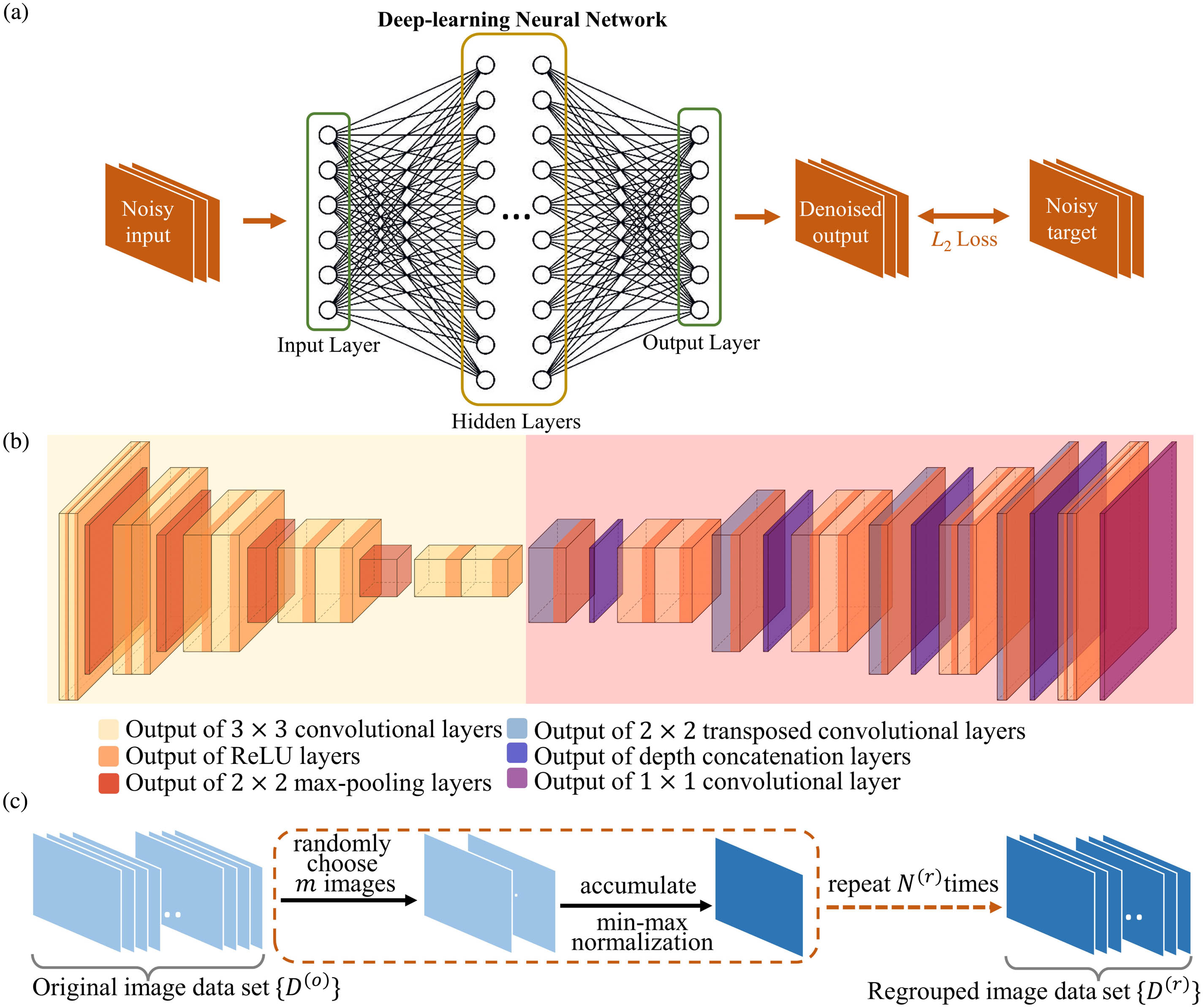
Fig. 1. (a) Schematic of the noise2noise protocol. Both the inputs and targets during training are noisy data, and the loss function is L₂ loss. With this protocol, the well-trained DL neural network can denoise the input noisy signal. (b) Diagram model for U-net. The structure includes two parts: the contracting part (left yellow area) and the expansive part (right pink area). Each slab represents a layer in the neural network. Colors indicate different types of layers, as shown by legends. (c) Schematic of data set preparation process. First, we randomly choose m frames from the original image data set {D^(o)}. These frames generate a new image through accumulation and min-max normalization. This procedure is repeated N^(r) times to obtain the regrouped image data set, including N^(r) frames. Then, the new data set is used for training.

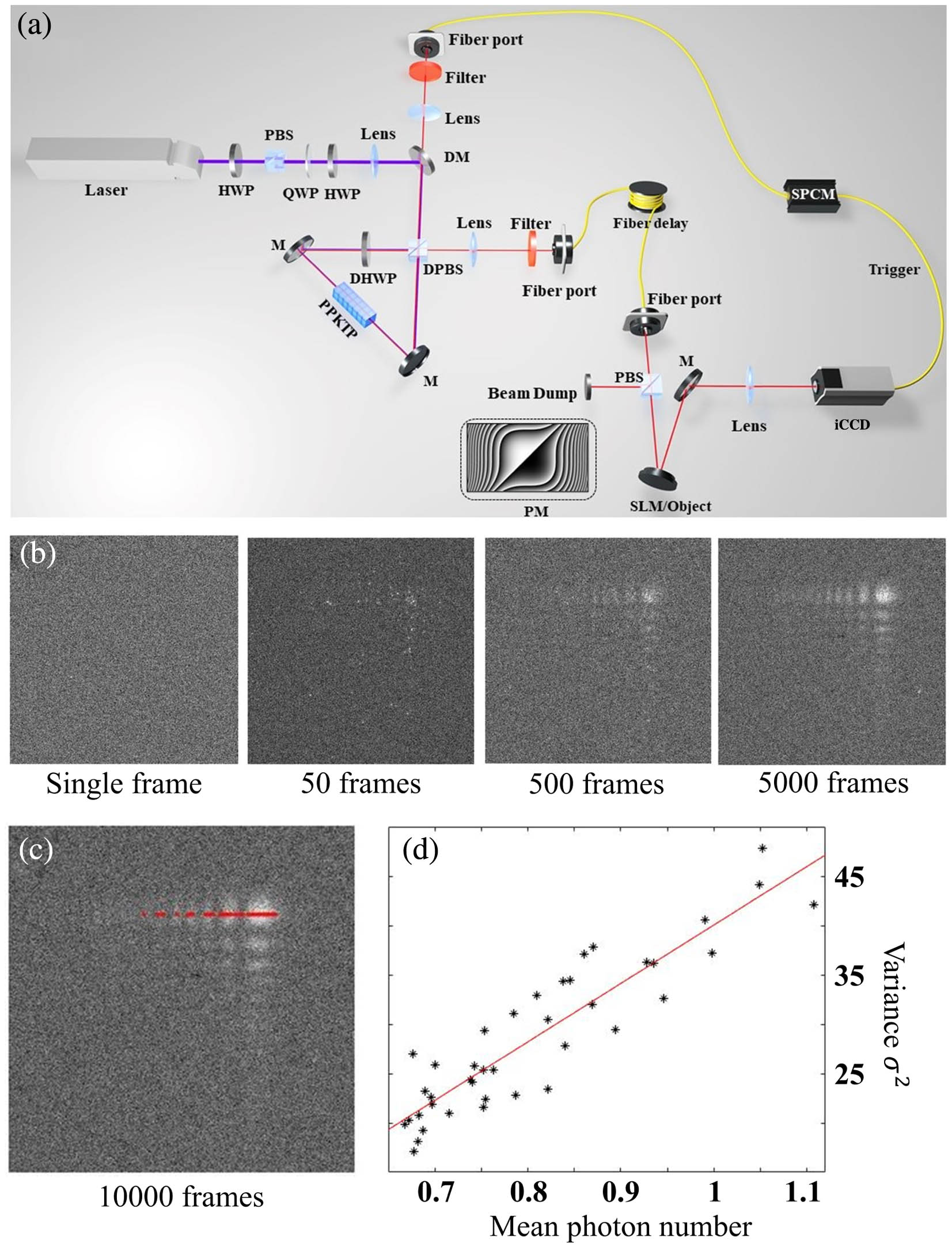
Fig. 2. Single-photon coincidence imaging of an Airy pattern. (a) Experimental setup. QWP, quarter-wave plate; HWP, half-wave plate; PBS, polarizing beam splitter; M, mirror; SPCM, single-photon counting module; PM, phase modulation; SLM, spatial light modulator; DM, dichroic mirror; DPBS, dual-wavelength PBS; DHWP, dual-wavelength HWP. An SLM is used as a scattering object to generate the Airy pattern. (b) Images accumulated over 1, 50, 500, and 5000 frames, respectively. The exposure time are Δt_e = 0.2 s. (c) Positions of the pixels (red points) that are chosen to calculate the variance in (d); (d) variance of the photon-number distribution versus the mean photon number n¯photon. A linear function (red line), σ2=59.19n¯photon−19.15, fits the variance well.

Fig. 3. Original and DL-enhanced Airy patterns for exposure time (a) Δt_e = 0.1 s and (b) 0.5 s, respectively; left column, top view of the original and DL-enhanced Airy patterns; middle column, projecting the Airy pattern to the y direction (side view); right column, brightness profiles along the red lines in the Airy pattern in left column. Red arrows are guides to the eye for the peaks appearing in the DL-enhanced images but indistinguishable in the original ones. Red curves in (b) represent the envelope of a theoretical Airy pattern.

Fig. 4. SNRs for the direct accumulation and the DL-based scheme. (a) Original image showing the areas for calculating SNR. The red dot indicates the center of the main peak of the Airy pattern. The red box surrounds a pure noise area. (b) SNR⁽¹⁾ versus the exposure time Δt_e; (c) SNR⁽²⁾ versus the regroup size m.