Surpassing the standard quantum limit of optical imaging via deep learning

Miao Cai; Zhi-Xiang Li; Hao-Dong Wu; Ya-Ping Ruan; Lei Tang; Jiang-Shan Tang; Ming-Yuan Chen; Han Zhang; Ke-Yu Xia; Min Xiao; Yan-Qing Lu

doi:10.3788/COL202321.082701

Abstract

The sensitivity of optical measurement is ultimately constrained by the shot noise to the standard quantum limit. It has become a common concept that beating this limit requires quantum resources. A deep-learning neural network free of quantum principle has the capability of removing classical noise from images, but it is unclear in reducing quantum noise. In a coincidence-imaging experiment, we show that quantum-resource-free deep learning can be exploited to surpass the standard quantum limit via the photon-number-dependent nonlinear feedback during training. Using an effective classical light with photon flux of about

9 \times 10^{4}

photons per second, our deep-learning-based scheme achieves a 14 dB improvement in signal-to-noise ratio with respect to the standard quantum limit.

Keywords

machine learning optical imaging standard quantum limit

1. Introduction

Optical measurement with sensitivity as high as possible is highly demanded in various science and technology, ranging from biology and astronomy to quantum information^[1–3]. However, the sensitivity of optical measurements is ultimately limited by the shot noise due to the quantum fluctuation of occupation of the probe field, imposing a constraint on the standard quantum limit (SQL) to the sensitivity limit^[4–8]. Quantum resources such as squeezed quantum states^[2,3,9–12] and highly entangled states^[13–16] have been proposed and successfully used to improve the measurement sensitivity beyond the SQL. Squeezed vacuum fields have also been exploited to reduce the noise level below the SQL in optical interferometers^[3,10]. Nevertheless, the squeezing-resulting improvement is easily destroyed by loss and phase noise. Thus, a deeply squeezed light is required to achieve a sensitivity far beyond the SQL but is very challenging to be prepared for a strong light. Alternatively, weak measurements^[17–20] have been proposed for beating the SQL in special circumstances. A nonlinear interferometer combined with quantum entanglement can even beat the Heisenberg limit of measurement^[2,21–25]. It is desirable to develop an approach for surpassing the SQL within a broadband and valid for a strong light including a huge number of photons.

Deep learning (DL) has become the working horse of improving performance of pattern recognition^[26,27], quantum information technology^[28], and imaging^[29–32]. DL mathematically treats noise as a random fluctuation of signals and has demonstrated the capability of beating some fundamental limit in physics such as the diffraction limit^[30,33]. Note that machine learning has been exploited to achieve a sensitivity scaling better than the SQL. Nevertheless, it still requires entangled qubits in measurement^[34]. Here we show that a DL neural network with the “noise2noise” protocol can suppress quantum noise without prior knowledge of a clean signal. Our work, which is free of using quantum entanglement or squeezing of the probe field such as entanglement or squeezing, provides a general approach to beat the SQL in the classical regime.

2. DL-Based Denoising Protocol

In the mathematical sense, DL can reduce random fluctuations of a detected signal, irrespective of the origin of the noise. Considering that the obtained signal is noisy in the practical measurement, we utilize the so-called noise2noise DL protocol, which can exploit the noisy signal as a target to reduce the noise in detection. In principle, a neural network depicted in Fig. 1(a) can be modeled as a regressor function $f_{θ}$ , where $θ$ is the network parameter set. After the DL network is fed with a set of data pairs ${({\hat{x}}_{i}, {\hat{y}}_{i})}$ of noisy inputs ${{\hat{x}}_{i}}$ and noisy targets ${{\hat{y}}_{i}}$ , the regressor function $f_{θ}$ and its parameter set ${θ}$ can be determined by the training process. The basic idea of neural network training is to minimize error between the network outputs and the given targets. The training process can generally be mathematically described as $f_{θ} = \underset{θ}{\arg \min} \sum_{i} L (f_{θ} ({\hat{x}}_{i}), {\hat{y}}_{i})$ , where $L$ is the loss function measuring error between the network output and the target. By specifying this loss function as a $L_{2}$ loss function, namely the least squared error, we exploit the DL noise2noise protocol.

Sign up for Chinese Optics Letters TOC. Get the latest issue of Chinese Optics Letters delivered right to you！Sign up now

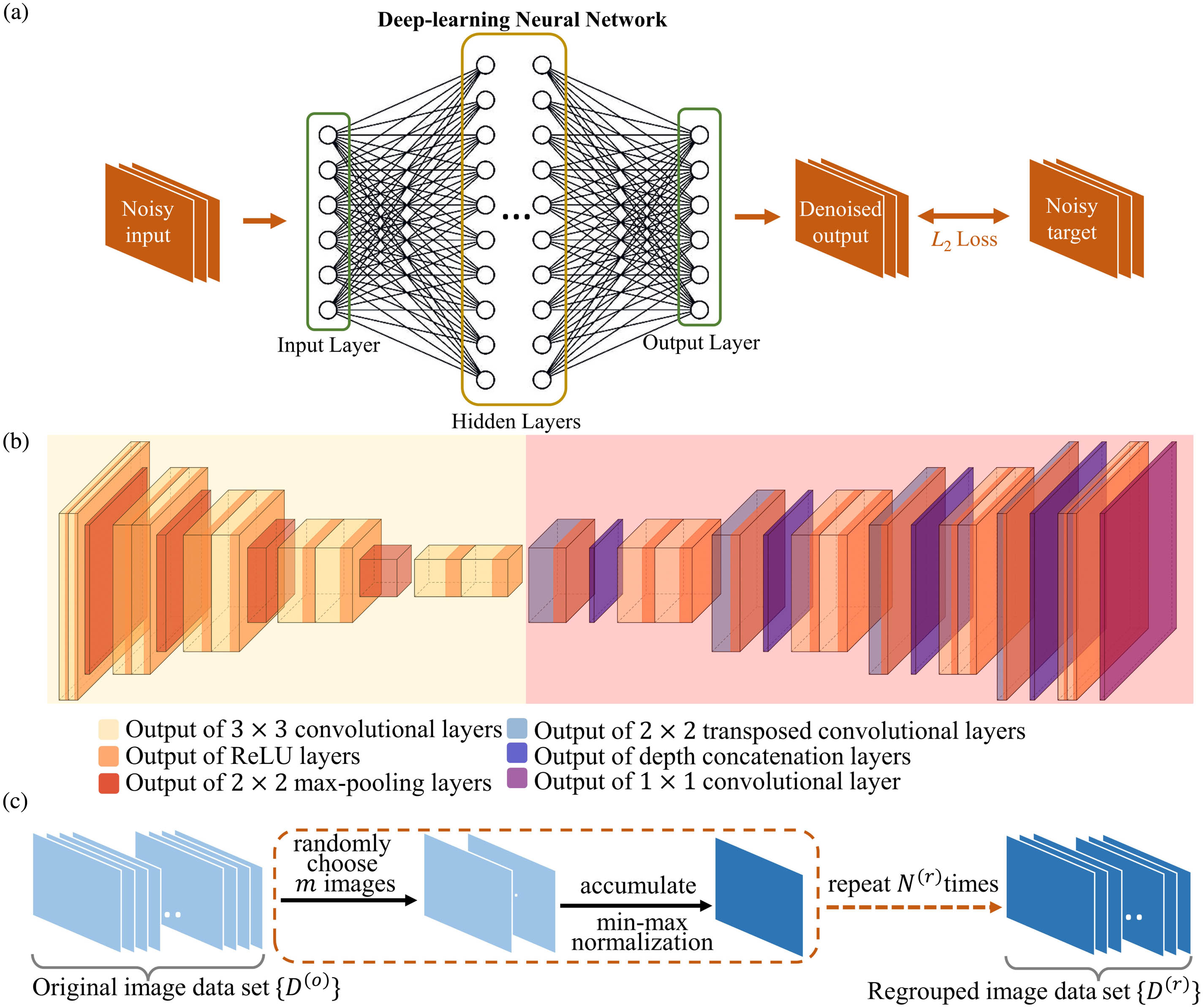
Figure 1.(a) Schematic of the noise2noise protocol. Both the inputs and targets during training are noisy data, and the loss function is L₂ loss. With this protocol, the well-trained DL neural network can denoise the input noisy signal. (b) Diagram model for U-net. The structure includes two parts: the contracting part (left yellow area) and the expansive part (right pink area). Each slab represents a layer in the neural network. Colors indicate different types of layers, as shown by legends. (c) Schematic of data set preparation process. First, we randomly choose m frames from the original image data set {D^(o)}. These frames generate a new image through accumulation and min-max normalization. This procedure is repeated N^(r) times to obtain the regrouped image data set, including N^(r) frames. Then, the new data set is used for training.

We now explain how a neural network with the noise2noise protocol can be used to suppress the shot noise and subsequently beat the SQL in measurement. We consider an observed imaging $r$ with noise in our optical measurement given by^[35] $r = s + p (s) + n,$ (1)where $s$ stands for the real signal of interest, $p (s)$ represents the shot noise, and $n$ stands for other system noise, such as the dark current noise and the readout noise. Note that both the dark current noise and the readout noise are statistically independent of the real signal. One can always set their mean values to zero via background subtraction. Thus, we can assume that $n$ satisfies the zero-mean condition without loss of generality. On the other hand, the shot noise $p (s)$ is theoretically a quantum fluctuation of received photon numbers. The probe signal with the fluctuation, $s + p (s)$ , obeys the Poisson distribution. We are interested in the signal $s$ , which is actually the averaged photon number and thus has no fluctuation. The distribution of the fluctuation $p (s)$ , denoting the shot noise in measurement, can be considered as a shifted Poisson distribution with zero-mean value.

In the noise2noise protocol, the input and target data sets are noisy data sets ${r_{input}}$ and ${r_{target}}$ , respectively. Then, we can mathematically describe the training process of the DL neural network with $L_{2}$ loss as $f_{θ - trained} = \underset{θ}{\arg \min} \sum_{i} {[f_{θ} (r_{input}) - r_{target}]}^{2},$ (2)where $f_{θ}$ and $f_{θ - trained}$ are the network functions during training and after training, respectively. $f_{θ}$ updates during the training process. By substituting Eq. (1) into Eq. (2), we obtain $f_{θ - trained} = \underset{θ}{\arg \min} \sum_{i} {f_{θ} [s + p_{input} (s) + n_{input}] - [s + p_{target} (s) + n_{target}]}^{2} .$ (3)

To minimize the loss in Eq. (3), $f_{θ - trained}$ needs to satisfy $f_{θ - trained} [s + p_{input} (s) + n_{input}] \sim E [s + p_{target} (s) + n_{target}] \sim s,$ (4)where the function $E$ calculates the ensemble moment. Equation (4) holds because both $p (s)$ and $n$ are the zero-mean distributions. This DL training process implicitly includes an extremely nonlinear feedback dependent on photon number “seen” by pixels. Thus, all types of noise in optical measurement can be reduced with our DL neural network.

Importantly, the nonlinear feedback enables the DL neural network to surpass the SQL for optical imaging. Physically, the probe field seen by a pixel collapses to a photon number state during each measurement. The photon number state can vary pixel by pixel and also fluctuate as measurement is ongoing. This fluctuation includes the shot noise and leads to the quantum standard limit in classical optical measurement. Now, we consider our DL-enhanced imaging. Assuming the original imaging has reached the standard quantum limit, which is reasonable in this coincidence imaging, the obtained image frame during each measurement can be modeled as $r_{m} (l, q) = P_{Poisson} [N_{m} \cdot P_{pattern} (l, q)],$ (5)where $r_{m}$ represents the obtained image frame of the $m$ th measurement, $l$ and $q$ are the pixel locations on the optical imaging device, $N_{m}$ is the total number of photons received by imaging device in the $m$ th measurement, and $P_{pattern}$ denotes the ideal pattern of photon distribution. Equation (5) indicates that the photon number on each pixel at $(l, q)$ obeys the Poisson distribution with a moment $λ_{Poisson} = N_{m} \cdot P_{pattern} (x, y)$ .

After the training is completed, for new input data $r_{m}^{'} (l^{'}, q^{'})$ at pixel $(l^{'}, q^{'})$ , the DL neural network returns an output as $f_{θ - trained} [r_{m}^{'} (l^{'}, q^{'})] = P_{output} [N_{m} \cdot P_{pattern} (l^{'}, q^{'})] .$ (6)

Here $P_{output}$ represents the photon number distribution given by well-trained DL network and is different from that of $r_{m} (l, q)$ because of the nonlinear feedback. With the training process of Eq. (2), the $L_{2}$ loss between $P_{output}$ and $P_{Poisson}$ is as small as possible. Then, the variance of $P_{output}$ , meaning the suppressed noise, can reduce to a level well below the shot noise.

This work shows the capability of using the noise2noise-based DL scheme to surpass the SQL in practical imaging. Note that optical imaging here, surpassing the SQL means to improve the signal-to-noise ratio (SNR) above the constraint imposed by the shot noise, when the overall number of photons is fixed during measurement. In practical measurement, the traditional noise2clean-based DL denoising approach may use the averaged image with a long exposure time as the clean target image. The available maximal SNR is up to that of the averaged image. These traditional methods need more photons or quantum resources. Therefore, they cannot surpass the SQL.

We used an end-to-end DL neural network, called U-net^[36]. The specific structure of the U-net is shown in Fig. 1(b). It includes two parts: the contracting path (yellow area) and the expansive path (pink area). The contracting path consists of four repeating encoder units. Each encoder unit has five layers: two $3 \times 3$ convolutional layers followed by a rectified linear unit (ReLU), and a $2 \times 2$ max pooling layer as the encoder unit. The contracting path extracts a multiscale latent representation of the input image. The expansive path also consists of four repeating decoder units. Each decoder units has seven layers: two $3 \times 3$ convolutional layers, each followed by a ReLU, one $2 \times 2$ transposed convolutional layer followed by a ReLU, and then a depth concatenation layer. In the end of the expansive path, there is a $1 \times 1$ convolutional layer as the final output layer. This comprehensive expansive path decompresses the representation from the contracting path to complete an end-to-end DL of target images.

Our DL-based denoising scheme can be divided into two stages: data preparation and training. The data preparation stage is depicted in Fig. 1(c). The $i$ th frame original image data obtained in experiment are denoted as ${D_{i}^{(o)}}$ with $i = {1,2,…, N^{(o)}}$ , where $N^{(o)}$ is the total number of image frames. In our experiment, we conduct the single-photon coincidence imaging with heralded single photons. Each original image frame only contains a few photons and is unsuitable for neural network training. In the data preparation stage, we randomly choose $m$ frames with equal probability from ${D^{(o)}}$ and then accumulate them into a new image frame. We apply min-max normalization on it. This procedure is repeated $N^{(r)}$ times. In doing so, we obtain a new image data set ${D^{(r)}}$ consisting of $N^{(r)}$ image frames. This new data set is equally divided into an input set and a target set. Each input frame corresponds to a target frame to form a noise2noise training pair. These pairs are then used in the training of the U-net. The training procedure updates the weights of the DL neural network. Once training finishes, we accumulate all the well-trained output image frames into the final denoised image. Our U-net training process is performed on an Intel Xeon Platinum 8180 CPU with MATLAB R2021a (see detailed hyperparameters in Appendix B).

3. Experimental Setup for Coincidence Imaging

We experimentally validate the suppression of the shot noise by using a DL neural network with the noise2noise DL protocol in single-photon coincidence imaging. Our experimental setup for generating the single-photon Airy pattern in each shot is shown in Fig. 2(a). We generate polarization-entangled heralded single photons from a spontaneous parametric downconversion process in a Sagnac interferometer embedded with a PPKTP crystal^[37]. The generation rate of correlated photon pairs is 9 kHz with a 5-ns coincidence measurement time window. Signal photons generated from the spontaneous parametric downconversion process are coupled out from an optical fiber with a fiber port and then pass through a polarizing beam splitter. After that, these single photons are incident on a reflective spatial light modulator (SLM) with the desired cubic phase modulation. The SLM generates the Airy pattern at the focal plane of lens $L$ . Generally, this SLM can be replaced with any scattering objects. Idler photons are collected to trigger the iCCD for detection of signal photons. The optical gate width of iCCD is set as 5 ns. The iCCD is in the integrate-on-chip mode with an exposure time $Δ t_{e}$ , which determines the accumulating period of signal photons before the imaging is read out. A 22-m-long optical fiber is used as a delay line to compensate for the electric delay of the iCCD. This ensures that signal photons reach the camera at the same time when the camera is triggered by the heralding detection of idler photons, which is in temporal correlation with signal photons. To make a convincing comparison between the shot noise and our DL-enhanced results, we use a trivial coincidence imaging to mimic the background noise other than the shot noise by switching on the time gate of the iCCD only when signal photons arrive. In our setup, signal photons are scattered by the object and directly detected by the iCCD. Thus, our arrangement is essentially different from the standard ghost imaging, in which photons in the scattering path are detected for triggering the detection of reference photons^[38,39]. Here, the temporal correlation between idler and signal photons is explored to generate a gate signal for switching on the iCCD. It can be replaced with an electric gate signal if coherent laser pulses are used for imaging.

Figure 2.Single-photon coincidence imaging of an Airy pattern. (a) Experimental setup. QWP, quarter-wave plate; HWP, half-wave plate; PBS, polarizing beam splitter; M, mirror; SPCM, single-photon counting module; PM, phase modulation; SLM, spatial light modulator; DM, dichroic mirror; DPBS, dual-wavelength PBS; DHWP, dual-wavelength HWP. An SLM is used as a scattering object to generate the Airy pattern. (b) Images accumulated over 1, 50, 500, and 5000 frames, respectively. The exposure time are Δt_e = 0.2 s. (c) Positions of the pixels (red points) that are chosen to calculate the variance in (d); (d) variance of the photon-number distribution versus the mean photon number ${\bar{n}}_{photon}$ . A linear function (red line), $σ^{2} = 59.19 {\bar{n}}_{photon} - 19.15$ , fits the variance well.

4. Beating the Shot Noise with DL

The small value of the conditional second-order correlation function clearly shows that the heralded single-photon source has a good single-photon nature and the two- or multiphoton events can be neglected (see details in Appendix A). The coincidence imaging is conducted in the setup shown in Fig. 2(a). Figure 2(b) shows the observed image accumulated over a single frame, 50 frames, 500 frames, and 5000 frames, respectively. For each frame, the exposure time is $Δ t_{e} = 0.2 s$ . These images clarify the single-photon coincidence imaging.

We first characterize noise in our experiment. According to Ref. [40], the shot noise $N_{shot}$ of a light field detected by the iCCD can be described as $N_{shot} = G \times F \times \sqrt{η ϕ_{p} Δ t_{e}},$ (7)where $G$ , $F$ , and $η$ are, respectively, the electron gain factor, the noise factor, and quantum efficiency. $ϕ_{p}$ is the mean photon flux of the light beam incident to each pixel, and $Δ t_{e}$ indicates the integration time in photon detection. Both dark current noise and readout noise are irrelevant with $ϕ_{p}$ . The total noise $N_{\exp}$ detected by each pixel dominantly attributes to the shot noise, dark current noise, and readout noise, respectively. We have $N_{\exp} = \sqrt{σ^{2}}$ , where $σ^{2}$ is the variance of observed pixel brightness. Therefore, if the experimental system reaches the shot-noise limit, $σ^{2}$ is linearly dependent on $ϕ_{p}$ when $Δ t_{e}$ is fixed.

Figures 2(c) and 2(d) confirm that our experiment is shot-noise-limited. In experiment, the exposure time of each frame is set to $Δ t_{e} = 0.2 s$ . We collect 10,000 original imaging frames. As shown in Fig. 2(c), we choose 100 pixels indicated by the red dots in all 10,000 frames to calculate the mean photon flux $ϕ_{p}$ and the corresponding noise variance $σ^{2}$ . The results are shown in Fig. 2(d). Clearly, the variance $σ^{2}$ increases linearly with $ϕ_{p} Δ_{e}$ . The value of the mean phonon number ${\bar{n}}_{photon}$ is the original readout brightness of the iCCD. It is proportional to the “real” photon number, according to the working mechanism of the iCCD. This verifies that our experiment system is shot-noise-limited.

Figure 3 shows that our DL algorithm can greatly reduce the noise of imaging. We measure the single-photon Airy pattern with $Δ t_{e} = 0.1 s$ and 0.5 s, respectively. For each $Δ t_{e}$ , the data set consists of 5000 original frames. The experimental images are directly accumulated from the original data set and then min-max normalized. They are equivalent to the standard averaged results, being subject to the SQL. To obtain DL-enhanced images, we create the training data set according to the procedure depicted in Fig. 1(c) with parameters $m = 500$ and $N^{(r)} = 1500$ . Then, this data set is fed into the neural network. The top and side views of the experimental and DL-enhanced images are illustrated in the left and middle columns. Some subtle peaks are overwhelmed by strong noise in the original images and thus are indistinguishable. In contrast, our DL neural network considerably reduces the noise level and generates much clearer images. As a result, more details of the imaging structure, including the blur peaks, become distinguishable. The right-column plots show the profiles along the red lines in the Airy patterns. After denoising, the DL-enhanced results clearly display two and four more peaks in comparison with the original images. The middle column shows that the DL algorithm has significantly reduced the amplitude of noise in a signal-free area (e.g., pixel position in $x$ direction from 0 to 50). With the exposure time $Δ t_{e}$ increasing (see gray bars in right column of Fig. 6 in Appendix C), the noise level and variance of the directly accumulated images approach those of the DL-enhanced results, respectively. This implies that the DL algorithm can remarkably suppress the shot noise within the same measurement time. In Fig. 3(b), we also plot the envelope of the theoretical Airy pattern (see also Appendix D). It can be seen that the envelope of the DL-enhanced result is better fitted by the theoretical envelope because the shot noise is greatly reduced.

Figure 3.Original and DL-enhanced Airy patterns for exposure time (a) Δt_e = 0.1 s and (b) 0.5 s, respectively; left column, top view of the original and DL-enhanced Airy patterns; middle column, projecting the Airy pattern to the y direction (side view); right column, brightness profiles along the red lines in the Airy pattern in left column. Red arrows are guides to the eye for the peaks appearing in the DL-enhanced images but indistinguishable in the original ones. Red curves in (b) represent the envelope of a theoretical Airy pattern.

Figure 4 characterizes the denoising performance of our DL algorithm by comparing the SNR between the original and the DL-enhanced images. Here, we use two definitions for SNR. Both are widely used for evaluating the performance of measurement^[41]. The first type of SNR is defined as ${SNR}^{(1)} = 10 \lg (P_{signal} / σ_{noise}^{2}),$ (8)where $P_{signal}$ is the central pixel brightness of the main peak of the Airy pattern, indicated by a red dot in Fig. 4(a), and $σ_{noise}^{2}$ is the variance of the pure noise area indicated by the red box. Figure 4(b) shows the directly accumulated ${SNR}^{(1)}$ using the original and the DL-enhanced images versus the exposure time $Δ t_{e}$ . This ${SNR}^{(1)}$ in both imaging methods increases with the exposure time increasing. Because the original image is at the shot-noise level, its SNR definitely reaches the SQL. In contrast to the standard accumulation scheme, the DL-based scheme can greatly improve the SNR. Basically, the improvement increases as the exposure time increases, corresponding to an effectively stronger classical light beam used for imaging. This DL-based scheme surpasses the SQL by more than 15 dB when $Δ t_{e} = 0.5 s$ , corresponding to about 18,000 photons detected in each frame. This shows that a DL neural network can beat the SQL in measurement without requiring quantum resources such as entanglement and squeezing, or prior knowledge of signals.

Figure 4.SNRs for the direct accumulation and the DL-based scheme. (a) Original image showing the areas for calculating SNR. The red dot indicates the center of the main peak of the Airy pattern. The red box surrounds a pure noise area. (b) SNR⁽¹⁾ versus the exposure time Δt_e; (c) SNR⁽²⁾ versus the regroup size m.

The improvement provided by the DL-based scheme can be further verified with the second type of SNR, defined as ${SNR}^{(2)} = 10 \lg (P_{signal} / σ_{signal}^{2}),$ (9)where the variance $σ_{signal}^{2}$ is calculated from the central pixel brightness of the main peak in the regrouped data sets. To evaluate ${SNR}^{(2)}$ , we first measure $10^{4}$ original image frames under an exposure time of $Δ t_{e} = 0.2 s$ . Then, according to the data-preparation procedure, we create 10 regrouped data sets with a grouping size $m$ ranging from 100 to 1000. Each regrouped data set contains 3000 frames, yielding 1500 frame pairs. The DL algorithm is then applied to obtain the corresponding denoised data sets for each regrouped data set. The variance $σ_{signal}^{2}$ shown in Fig. 4(c) is calculated from the regrouped data set and the DL-enhanced data set, respectively. The DL-based scheme has significantly reduced the variance of the directly accumulated signal, indicating a great suppression of the shot noise. At $m {= 10}^{3}$ , the SNR is improved by about 14 dB. Because the observed signal’s variance represents the shot-noise level, the DL-based scheme clearly reaches an SNR far beyond the SQL. Each image in the regrouped data set is equivalent to an observation with an exposure time $m Δ t_{e}$ , varying from 20 to 200 s. In doing so, we equivalently conduct imaging with a classical coherent light including $7 \times 10^{5} - 7 \times 10^{6}$ photons in each frame (see Appendix A).

5. Conclusion and Discussion

In summary, we have proposed and demonstrated a DL-based denoising scheme to achieve measurement sensitivity beyond the SQL with only a classical resource. The photon-number-dependent nonlinear feedback during training significantly suppresses the shot noise inherently existing in measurement. This work opens the door to achieve unprecedented precision in measurement. Meanwhile, the data postprocessing nature of our scheme makes it generally valid for various measurement systems. This DL-based denoising scheme is not limited to optical imaging but is also applicable to spectroscopy and various interferometers. It can even be extended to the microwave and acoustic-wave domains.

References

[1] Y. M. Sigal, R. Zhou, X. Zhuang. Visualizing and discovering cellular structures with super-resolution microscopy. Science, 361, 880(2018).

[2] C. A. Casacio, L. S. Madsen, A. Terrasson, M. Waleed, K. Barnscheidt, B. Hage, M. A. Taylor, W. P. Bowen. Quantum-enhanced nonlinear microscopy. Nature, 594, 201(2021).

[3] J. Aasi, J. Abadie, D. A. Brown. Enhanced sensitivity of the LIGO gravitational wave detector by using squeezed states of light. Nat. Photonics, 7, 613(2013).

[4] V. B. Braginsky, Y. I. Vorontsov. Quantum-mechanical limitations in macroscopic experiments and modern experimental technique. Sov. Phys. Usp., 17, 644(1975).

[5] V. Giovannetti, S. Lloyd, L. Maccone. Quantum-enhanced measurements: beating the standard quantum limit. Science, 306, 1330(2004).

[6] K. Xia, N. Zhao, J. Twamley. Detection of a weak magnetic field via cavity-enhanced Faraday rotation. Phys. Rev. A, 92, 043409(2015).

[7] J. P. Dowling. Correlated input-port, matter-wave interferometer: Quantum-noise limits to the atom-laser gyroscope. Phys. Rev. A, 57, 4736(1998).

[8] S. Schreppler, N. Spethmann, N. Brahms, T. Botter, M. Barrios, D. M. Stamper-Kurn. Optically measuring force near the standard quantum limit. Science, 344, 1486(2014).

[9] C. M. Caves. Quantum-mechanical radiation-pressure fluctuations in an interferometer. Phys. Rev. Lett., 45, 75(1980).

[10] M. Xiao, L.-A. Wu, H. J. Kimble. Precision measurement beyond the shot-noise limit. Phys. Rev. Lett., 59, 278(1987).

[11] H. Vahlbruch, M. Mehmet, S. Chelkowski, B. Hage, A. Franzen, N. Lastzka, S. Gossler, K. Danzmann, R. Schnabel. Observation of squeezed light with 10-db quantum-noise reduction. Phys. Rev. Lett., 100, 033602(2008).

[12] K. Xia, J. Twamley. Generating spin squeezing states and Greenberger-Horne-Zeilinger entanglement using a hybrid phonon-spin ensemble in diamond. Phys. Rev. B, 94, 205118(2016).

[13] S. Haine, A. Ferris. Surpassing the standard quantum limit in an atom interferometer with four-mode entanglement produced from four-wave mixing. Phys. Rev. A, 84, 043624(2011).

[14] L.-Z. Liu, Y.-Z. Zhang, Z.-D. Li, R. Zhang, X.-F. Yin, Y.-Y. Fei, L. Li, N.-L. Liu, F. Xu, Y.-A. Chen, J.-W. Pan. Distributed quantum phase estimation with entangled photons. Nat. Photonics, 15, 137(2021).

[15] T. Nagata, R. Okamoto, J. L. O’Brien, K. Sasaki, S. Takeuchi. Beating the standard quantum limit with four-entangled photons. Science, 316, 726(2007).

[16] C. Gross, T. Zibold, E. Nicklas, J. Esteve, M. K. Oberthaler. Nonlinear atom interferometer surpasses classical precision limit. Nature, 464, 1165(2010).

[17] M. F. Bocko, R. Onofrio. On the measurement of a weak classical force coupled to a harmonic oscillator: experimental progress. Rev. Mod. Phys., 68, 755(1996).

[18] V. B. Braginsky, F. Y. Khalili. Quantum nondemolition measurements: the route from toys to tools. Rev. Mod. Phys., 68, 1(1996).

[19] G. Chen, P. Yin, W.-H. Zhang, G.-C. Li, C.-F. Li, G.-C. Guo. Beating standard quantum limit with weak measurement. Entropy, 23, 354(2021).

[20] K. Xia, M. Johnsson, P. L. Knight, J. Twamley. Cavity-free scheme for nondestructive detection of a single optical photon. Phys. Rev. Lett., 116, 023601(2016).

[21] M. Napolitano, M. Koschorreck, B. Dubost, N. Behbood, R. Sewell, M. W. Mitchell. Interaction-based quantum metrology showing scaling beyond the Heisenberg limit. Nature, 471, 486(2011).

[22] J. Joo, W. J. Munro, T. P. Spiller. Quantum metrology with entangled coherent states. Phys. Rev. Lett., 107, 083601(2011).

[23] S. Boixo, A. Datta, M. J. Davis, S. T. Flammia, A. Shaji, C. M. Caves. Quantum metrology: dynamics versus entanglement. Phys. Rev. Lett., 101, 040403(2008).

[24] C.-P. Wei, Z.-M. Zhang. Improving the phase sensitivity of a Mach–Zehnder interferometer via a nonlinear phase shifter. J. Mod. Opt., 64, 743(2017).

[25] N. Treps, U. Andersen, B. Buchler, P. K. Lam, A. Maitre, H.-A. Bachor, C. Fabre. Surpassing the standard quantum limit for optical imaging using nonclassical multimode light. Phys. Rev. Lett., 88, 203601(2002).

[26] A. Shrestha, A. Mahmood. Review of deep learning algorithms and architectures. IEEE Access, 7, 53040(2019).

[27] M. Paolanti, E. Frontoni. Multidisciplinary pattern recognition applications: a review. Comput. Sci. Rev., 37, 100276(2020).

[28] M. Cai, Y. Lu, M. Xiao, K. Xia. Optimizing single-photon generation and storage with machine learning. Phys. Rev. A, 104, 053707(2021).

[29] J. Xie, L. Xu, E. Chen. Image denoising and inpainting with deep neural networks. Adv. Neural Inf. Process Syst., 25, 341(2012).

[30] L. Tian, L. Waller. 3D intensity and phase imaging from light field measurements in an LED array microscope. Optica, 2, 104(2015).

[31] C. Tian, L. Fei, W. Zheng, Y. Xu, W. Zuo, C.-W. Lin. Deep learning on image denoising: An overview. Neural Netw., 131, 251(2020).

[32] F. Wang, C. Wang, M. Chen, W. Gong, Y. Zhang, S. Han, G. Situ. Far-field super-resolution ghost imaging with a deep neural network constraint. Light Sci. Appl., 11, 1(2022).

[33] P. R. Wiecha, A. Lecestre, N. Mallet, G. Larrieu. Pushing the limits of optical information storage using deep learning. Nat. Nanotechnol., 14, 237(2019).

[34] A. Hentschel, B. C. Sanders. Machine learning for precise quantum measurement. Phys. Rev. Lett., 104, 063603(2010).

[35] J. J. Heine, M. Behera. Aspects of signal-dependent noise characterization. J. Opt. Soc. Am. A, 23, 806(2006).

[36] O. Ronneberger, P. Fischer, T. Brox. U-net: convolutional networks for biomedical image segmentation. International Conference on Medical image computing and computer-assisted intervention, 234(2015).

[37] Z.-X. Li, Y.-P. Ruan, J. Tang, Y. Liu, J.-J. Liu, J.-S. Tang, H. Zhang, K.-Y. Xia, Y.-Q. Lu. Self-healing of a heralded single-photon Airy beam. Opt. Express, 29, 40187(2021).

[38] R. S. Bennink, S. J. Bentley, R. W. Boyd. ‘Two-photon’ coincidence imaging with a classical source. Phys. Rev. Lett., 89, 113601(2002).

[39] R. S. Bennink, S. J. Bentley, R. W. Boyd. Quantum and classical coincidence imaging. Phys. Rev. Lett., 92, 033601(2004).

[40] D. Dussault, P. Hoess. Noise performance comparison of ICCD with CCD and EMCCD cameras. Proc. SPIE, 5563, 195(2004).

[41] D. J. Schroeder. Astronomical Optics(1999).