Experimental demonstration of full-field quantum optical coherence tomography

Zeferino Ibarra-Borja; Carlos Sevilla-Gutiérrez; Roberto Ramírez-Alarcón; Hector Cruz-Ramírez; Alfred B. U’Ren

doi:10.1364/PRJ.8.000051

Abstract

We present, to the best of our knowledge, the first implementation of full-field quantum optical coherence tomography (FF-QOCT). In our system, we are able to obtain full three-dimensional (3D) information about the internal structure of a sample under study by relying on transversely resolved Hong–Ou–Mandel (HOM) interferometry with the help of an intensified CCD (ICCD) camera. Our system requires a single axial scan, obtaining full-field transverse single-photon intensity in coincidence with the detection of the sibling photon for each value of the signal-idler temporal delay. We believe that this capability constitutes a significant step forward toward the implementation of QOCT as a practical biomedical imaging technique.

1. INTRODUCTION

Optical coherence tomography (OCT) [1,2] is a valuable imaging technique capable of producing three-dimensional (3D) ( $x - y$ transverse, $z$ axial), high-resolution images revealing the internal structure of inhomogeneous samples, such as biological tissue, with an axial resolution in the region of 0.75–20 μm and penetration depths around 1–3 mm [3,4]. OCT is based on low-coherence interferometry and employs a short-coherence-time light source propagating in a Michelson interferometer to carry out axial sectioning of a specimen. Unfortunately, increasing the source bandwidth in OCT to achieve a higher axial resolution, on the contrary, can result in a degraded resolution due to group velocity dispersion (GVD) in the medium [5].

By exploiting fundamental properties of quantum states of light, a promising technique arises in the form of quantum optical coherence tomography (QOCT), which is based on Hong–Ou–Mandel interference (HOM) between photon pairs generated through the process of spontaneous parametric down-conversion (SPDC) [6,7]. In QOCT, one of the photons in each pair is reflected from the sample under study before meeting its sibling photon at a beamsplitter (BS). Remarkably, QOCT provides a factor of 2 enhancement in axial resolution, with respect to an equivalent classical system with the same bandwidth [7–9]. For a sufficiently narrow SPDC pump bandwidth it is inherently immune to even-order dispersion effects in the sample, including GVD [10–12]. QOCT axial resolutions down to the sub-μm level are possible through appropriate engineering of the photon pair source [13,14].

We note that some recent advances have extended the capabilities of (classical) OCT configurations. For instance, by reducing the central wavelength of the radiation, instead of increasing the bandwidth, recent work based on broadband ultraviolet and X-ray sources has shown extreme resolutions down to 2 nm for the so-called silicon and water windows [15,16]. In a different approach, by exploiting the effect of induced coherence produced in nonclassical radiation generated by a parametric down-conversion (PDC), it is possible to implement a versatile OCT configuration where photons in the infrared region interact with a sample, but the detection is conveniently carried out with the sibling photons in the visible region [17,18].

Sign up for Photonics Research TOC. Get the latest issue of Photonics Research delivered right to you！Sign up now

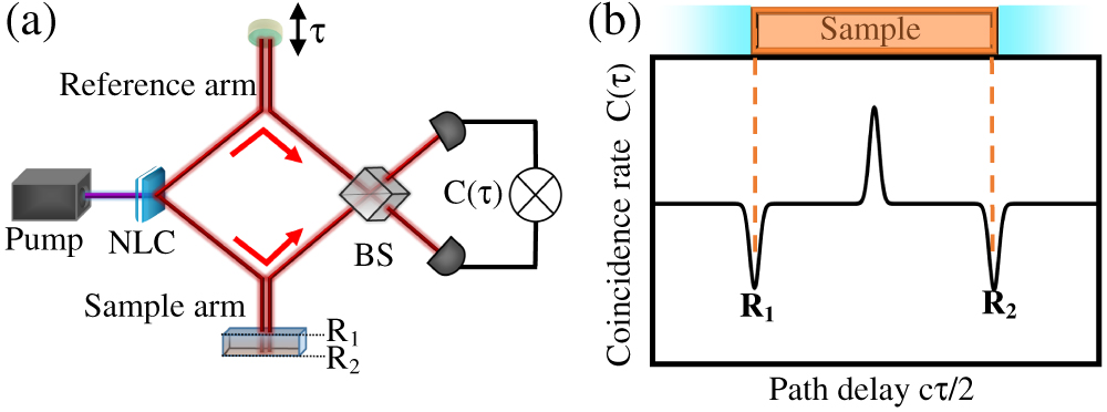
In a typical QOCT configuration, noncollinear SPDC photon pairs are used, with the signal and idler modes defining the reference and sample arms (see Fig. 1). The idler photon in the reference arm is reflected by a mirror mounted on a translation stage, which introduces a controlled temporal delay $τ$ , while the signal photon interacts with the sample being reflected from the various interfaces associated with its internal structure. The two photons are then directed to the input ports of a nonpolarizing 50:50 BS, where the HOM interference effect occurs. The two output ports then lead to appropriate single-photon detectors to monitor the resulting coincidence count rate $C (τ)$ , as defined below.

(a) Standard configuration for QOCT based on HOM interference. (b) Typical QOCT interferogram, based on an A-scan, for a two-layer sample with reflectivities R1 and R2.

Figure 1.(a) Standard configuration for QOCT based on HOM interference. (b) Typical QOCT interferogram, based on an A-scan, for a two-layer sample with reflectivities $R_{1}$ and $R_{2}$ .

For a sample containing a single interface (i.e., a standard mirror), a single HOM dip appears centered at the position that yields $τ = 0$ . If multiple interfaces are present in the sample, each will produce an HOM dip, while in addition cross-interference terms will appear for each pair of interfaces. A full scan of the mirror along $z$ (referred to as an A-scan), will reveal these various dips and cross-interference structures, which can be either in the form of a dip or a peak [19]. An illustration based on a two-layer sample is shown in Fig. 1(b). In QOCT, the positions of the dips are used to reconstruct the axial structure of the sample at a particular transverse ${x, y}$ position in the sample. A 3D sectioned reconstruction of the sample can be obtained by scanning the sample transversely on a two-dimensional (2D) $x - y$ grid (referred to as a C-scan), for each axial position $z$ in the A-scan.

Such a 3D reconstruction, formed by the stacking of multiple C-scans (one per axial position), would be extremely time consuming [1,9,20]. In the case of (classical) OCT, techniques have been demonstrated that optimize this process, such as Fourier domain OCT (FD-OCT), which eliminates the need for mechanical axial scanning [21], and full-field OCT (FF-OCT), which uses a CCD camera to eliminate the need for transverse scanning [22,23]. Note that thanks to their ns gating capabilities and high quantum efficiencies, intensified CCD (ICCD) cameras recently have increased the versatility of quantum imaging experiments such as ghost imaging schemes [24,25] and also have enabled notable experiments such as the real-time imaging of quantum entanglement [26], the shot-by-shot imaging of quantum interference [27], and the observation of the hologram of a single photon [28].

In this paper we report on what we believe is the first implementation of full-field QOCT, in which we capture the full transverse $x - y$ field (C-scan) in a single shot, exploiting $1024 \times 1024$ pixels of an ICCD camera, allowing for 3D sectioned reconstruction of a sample through a single A-scan acquisition sequence. We have developed the ability to obtain a volumetric reconstruction of the internal structure of a sample, while (i) retaining the quantum-enabled improvement in axial resolution, and (ii) maintaining the acquisition time as short as possible through the exploitation of ICCD technology, thus taking QOCT one step closer to becoming a practical biomedical imaging technology.

2. THEORY

A sample under study in QOCT can be represented by the sample reflectivity function $H (ω)$ (SRF), which modifies the SPDC joint amplitude as a multiplicative factor and which, for the case of two-layers, can be written as [7,8,19] $H (ω) = r_{1} + r_{2} e^{i 2 ω n L / c},$ (1)where $R_{1} = {| r_{1} |}^{2}$ and $R_{2} = {| r_{2} |}^{2}$ are the reflectivities from the front and back surfaces; $ω$ is the frequency; $c$ is the speed of light in vacuum; $L$ is the thickness; and $n$ is the refractive index of the sample. $2 ω n L / c$ represents the phase accumulated by the photon in a round trip through the thickness of the sample. The QOCT interferogram $C (τ)$ obtained from an A-scan, normalized so that $C (τ) = 1$ for $τ \to \pm \infty$ , can be expressed as [8,19] $C (τ) \sim 1 - γ V_{1} s (2 τ) - γ V_{2} s (2 τ - 2 T) - γ V_{mid} s (2 τ - T),$ (2)in terms of the SPDC intensity envelope, $s (τ)$ , and the temporal layer separation $T = 2 n L / c$ , where $s (τ)$ is the Fourier transform of the SPDC spectral distribution function $S (ω)$ . The second and third terms in Eq. (2) are the HOM dips resulting from the front and back surfaces, with visibilities $V_{1}$ and $V_{2}$ , respectively. The last term, with an amplitude $V_{mid}$ , originates from cross-interference between both surfaces. Note that the factor of 2 in the argument of $s (τ)$ is responsible for the enhancement in axial resolution for QOCT, as compared to an equivalent classical setup [7]. $V_{1}$ , $V_{2}$ , and $V_{mid}$ are given by $V_{1} = \frac{R_{1}}{R_{1} + R_{2}}; V_{2} = \frac{R_{2}}{R_{1} + R_{2}}; V_{mid} = \frac{2 \sqrt{R_{1} R_{2}}}{R_{1} + R_{2}} \cos (ω_{0} T),$ (3)in terms of effective reflectivities $R_{1} = R_{1}$ and $R_{2} = {(1 - R_{1})}^{2} R_{2}$ , which quantify the relative flux participating in the HOM interference from each of the two surfaces. Note that the intermediate structure can be either a peak or a dip, as governed by $ω_{0} T$ (with $ω_{0}$ the SPDC pump frequency). The indistinguishability parameter $γ$ , which obeys $0 \leq γ \leq 1$ , results from the integral overlap of the interfering photon wave functions [29,30], and limits the visibility that can be obtained for each HOM dip in the QOCT interferogram. Note that its value can be obtained as the HOM visibility $γ = V$ resulting from a single-interface sample (i.e., a mirror). The dip visibilities obtained in the QOCT interferogram that is associated with the various layers will add up to $V$ [19].

3. EXPERIMENT

In our setup (see Fig. 2), the photon-pair source is based on a β barium borate (β-BBO) crystal of 2 mm thickness, cut at 29.2° for type-I phase matching. The crystal is pumped by a diode laser emitting at 403.6 nm with power of 50 mW, focused (with a lens L of $f = 1000 mm$ focal length) to a beam waist of $w_{0} \approx 300 μm$ at the crystal plane (BBO). This configuration produces noncollinear ( $\pm 3 °$ ), co-polarized, frequency-degenerate photon pairs.

Figure 2.(a) FF-QOCT setup. (b) Schematic of the sample used showing the empty frame and the frame with the letter $ψ$ imprinted on the front surface, along with the sample structure observed with a microscope. (c) Image-preserving OD.

For our experiments, we use two distinct spectral configurations for the photon pairs, as given by the spectral filter element (SFE): source configuration A (filtered) involving a long-pass filter that transmits wavelengths $λ > 500 nm$ (Thorlabs FELH0500), followed by a $810 \pm 5 nm$ bandpass filter (Thorlabs FBH810-10), and source configuration B (unfiltered) that involves only the long-pass filter. Note that source configuration B maximizes the SPDC bandwidth and also maximizes the achievable axial resolution in QOCT. Once being redirected by a triangular mirror (TM), the two photons define the reference and sample arms shown in Fig. 2.

To ensure spatial mode indistinguishability, we project both photons into Gaussian modes by coupling them with aspheric lenses ( ${AL}_{1}$ and ${AL}_{2}$ , $f = 8 mm$ ) into polarization-maintaining, single-mode fibers ( ${PMSMF}_{1}$ and ${PMSMF}_{2}$ ). At the output of the fibers the collimation is adjusted (with lenses ${AL}_{3}$ and ${AL}_{4}$ , $f = 8 mm$ ) to obtain modes with a beam diameter of $\sim 1 mm$ at the reference (M₁) and sample (SAMPLE) planes. The diameter of the Gaussian mode illuminating the sample defines the area of interest that will be captured by the ICCD camera (Andor iStar 334T).

The idler photon propagating through the reference arm is sent to the temporal delay system, composed of a polarization beamsplitter ( ${PBS}_{1}$ ), a quarter-wave plate ( ${QWP}_{1}$ ), and a mirror (M₁) mounted on a stepper motor with a minimum 100 nm step. A $1 \times$ 4f telescope, formed by plano-convex lenses $L_{1}$ ( $f = 150 mm$ ) and $L_{2}$ ( $f = 150 mm$ ), then creates an image of the idler photon spatial mode at M₁, on the plane of the non-polarizing BS, defining the image plane (IP). The signal photon propagating through the sample arm traverses an identical set of elements, except for the presence of the sample instead of a mirror. The photon then traverses a $1 \times$ 4f telescope formed by plano-convex lenses $L_{3}$ ( $f = 150 mm$ ) and $L_{4}$ ( $f = 150 mm$ ), creating an image of the signal photon spatial mode at the front surface of the sample, on the plane of the BS (IP). For values of the temporal delay, defined by the position of mirror M₁, which result in the temporal overlap of the two photons at the beamsplitter, the HOM interference effect occurs, revealing the presence of reflecting layers in the sample.

For each delay value $τ$ in a given A-scan, a full-field C-scan is obtained in a single shot by capturing the 2D single-photon transverse intensity distribution. Note that the ICCD camera used for this purpose is operated in a gated configuration, collecting single photons on path 3 in coincidence with the corresponding single photons on path 4 (with the BS output ports defining paths 3 and 4). Photons propagating through path 4 are coupled into a single-mode optical fiber ${SMF}_{2}$ (using aspheric lens ${AL}_{6}$ , $f = 8 mm$ ) leading to an avalanche photodiode ${APD}_{2}$ (Excelitas SPCM-AQRH). The transistor-transistor logic (TTL) output pulses from ${APD}_{2}$ are discriminated and delayed by a series of nuclear instrumentation standard module (NIM) elements and then used to trigger the ICCD camera, placed following an imaging-preserving $\sim 90 ns$ ( $\sim 28 m$ ) optical delay line (OD), designed to overcome the insertion delay of the ICCD [24]. Photons propagating along path 3 are transmitted through a telescope formed by plano-convex lenses $L_{5}$ ( $f = 60 mm$ ) and $L_{6}$ ( $f = 150 mm$ ), with a $2.5 \times$ magnification, prior to entering the OD built in a double-pass configuration that relays the magnified image from IP to the ICCD detection plane (DP).

In the OD, p-polarized photons from path 3 are transmitted by the PBSD, placed at the focal plane of the first $1 \times$ telescope, and formed by two bi-convex $2^{''}$ diameter, 500 mm focal length lenses ( ${LD}_{1}$ and ${LD}_{2}$ ). The photons then traverse three consecutive $1 \times$ 4f telescopes, formed by two bi-convex $2^{''}$ diameter, 1000 mm focal length lenses ( ${LD}_{3}$ through ${LD}_{8}$ ). A quarter-wave plate (QWPD) placed prior to mirror ${MD}_{7}$ rotates the polarization from p to s so that, on their way back, the photons propagate through the 1000 mm $1 \times$ 4f telescopes and then through the 500 mm $1 \times$ 4f telescope, except that they are now reflected at the PBSD, defining a new optical path which, with a third $2^{''}$ diameter 500 mm focal length lens ( ${LD}_{9}$ ), relays the propagated image to plane DP. As the OD preserves the $2.5 \times$ magnification from the input telescope, the transverse resolution obtained at the sample plane is $\sim 5.2 μm$ , as defined by the $13 μm \times 13 μm$ ICCD pixels.

The sample used in our experiments is a 12 mm-diameter, 174 μm-thickness borosilicate glass coverslip, with a refractive index $n = 1.51$ at 800 nm, to which a thin-film copper deposition was applied on both sides. The deposition was calculated to obtain $R_{1} = 0.45$ and $R_{2} = 0.8$ normal-incidence reflectivities from the front and back surfaces at 800 nm. We chose this combination of reflectivities to obtain a good contrast in the spatially resolved measurements by the FF-QOCT technique (see below). Using a femtosecond direct laser writing technique (FDLW) [31], we controllably damaged the thin film on the front surface, thus reducing its thickness, in specific user-selected regions. This process allows us to “print” an arbitrary design on the thin film with a lateral minimum thickness of 5 μm. We defined two $1500 μm \times 1500 μm$ frames on the front surface and imprinted a letter $ψ$ with dimensions $500 μm \times 400 μm$ on one of them, to be revealed by the FF-QOCT technique, while leaving the other frame undamaged or empty [Fig. 1(b)]. It should be mentioned that because imprinting occurs on a thin film with a thickness of a few nm, we do not expect to be able to resolve the topography (variation in thickness) of the sample [9]. Nevertheless, the sample used demonstrates our capability to: (i) acquire full-field C-scans in a single shot, and (ii) obtain a 3D sectioned reconstruction of the internal structure of the sample with a single A-scan acquisition sequence.

To test our setup, we initially carry out nontransversely resolved measurements for which we deviate photons in path 3 with a flipping mirror (FM), to be coupled with aspheric lens ${AL}_{5}$ ( $f = 8 mm$ ) into single-mode fiber ${SMF}_{1}$ and detected with ${APD}_{1}$ , instead of traversing the OD to reach the ICCD camera. First, we obtain a standard HOM dip by replacing the sample with a reflecting mirror identical to M₁ in Fig. 2. Second, we obtain the QOCT interferogram (A-scan) at a specific transverse location within the empty frame. In both of these measurements, we perform an A-scan acquisition sequence, which involves displacing M₁ along the $z$ direction with 0.5 μm steps, while monitoring the coincidence count rate $C (τ)$ between ${APD}_{1}$ and ${APD}_{2}$ with 1 s accumulation time and a 10 ns coincidence window. The coincidence counts (CC in Fig. 2) were registered by a time-to-digital converter module (ID Quantique id800). These test measurements were carried out for source configurations A and B (see above). While configuration A [Figs. 3(a) and 3(b)] optimizes the single-dip HOM visibility reaching $V_{A} = 95.5 %$ , with an axial resolution FWHM dip width of 33.4 μm, configuration B [Figs. 3(c) and 3(d)] improves the axial resolution down to 6.5 μm, by taking advantage of the full SPDC bandwidth, with a reduced visibility of $V_{B} = 66.3 %$ . The reduced visibility in configuration B is probably due to increased photon-pair distinguishability, which can result from joint spectral amplitude asymmetry within the broader spectrum of configuration B, and/or to a slight misalignment of the fiber tips of single-mode fibers, ${PMSMF}_{1}$ and ${PMSMF}_{2}$ , leading to a slight spectral shift in the signal and idler central frequencies.

Figure 3.For a single-layer sample (mirror): (a) and (c) experimental HOM dip for photon-pair source in configuration A (filtered), in panel (a), and for configuration B (unfiltered) in panel (c). The insets in panels (a) and (c) show the single-photon spectral distribution $S (ω)$ measured at the single-mode fiber outputs. Both distributions are approximately rectangular in shape with bandwidths $\sim 10 nm$ and $\sim 50 nm$ , respectively. For the empty frame in the sample: (b) and (d) experimental QOCT interferogram for configuration A (filtered), in panel (b), and for configuration B (unfiltered) in panel (d). The continuous lines are corresponding theory curves.

The QOCT interferogram measurements [see Figs. 3(b) and 3(d)] show the two characteristic dips corresponding to the two sample interfaces, separated by the optical path length ( $n L = 264 μm$ ), which also shows the intermediate structure due to cross-interference from both surfaces. Source configuration A leads to visibilities, $V_{A 1} = 62.3 %$ and $V_{A 2} = 32.8 %$ , for the front and back surfaces, respectively, while source configuration B leads to visibilities, $V_{B 1} = 45.2 %$ and $V_{B 2} = 21.4 %$ . Note that, as expected, $V_{A 1} + V_{A 2} \approx V_{A}$ and $V_{B 1} + V_{B 2} \approx V_{B}$ .

From the single-dip interferograms [see Figs. 3(a) and 3(c)], we can obtain the indistinguishability parameter $γ$ for each of the two source configurations, as $γ_{A} = V_{A}$ and $γ_{B} = V_{B}$ . Using these values for $γ$ in Eq. (2) along with the values for the other parameters already specified above, we obtain the theory curves shown in Figs. 3(b) and 3(d), exhibiting an excellent agreement with the experimental data. We note that the shape of the dips is governed by the SPDC spectral amplitude $S (ω)$ , which in our case is determined by a spectral filter with a roughly rectangular spectral profile, in both source configurations. This implies that function $s (τ)$ will exhibit sinc-style sidelobes, thus explaining the appearance of additional structures, resembling lower-visibility dips, placed symmetrically around each dip.

As a third, nontransversely resolved test of our setup, we compare the QOCT interferogram obtained with the signal photon being reflected from the sample in the regions with and without the letter $ψ$ imprinted. The results, shown in Fig. 4, show a slight variation between the two interferograms indicating that, while the QOCT A-scan can respond to differences in the transverse morphology between the two regions (with $ψ$ and no $ψ$ imprinted), it is evidently unable to give detailed information about the nature of such differences.

Figure 4.QOCT interferogram obtained for the sample when illuminating the empty frame (purple dots) and the frame containing the letter $ψ$ imprinted (green dots).

We will now turn our attention to our full transversely resolved FF-QOCT measurement, for which a C-scan is performed in a single shot at each delay value $τ$ of a single A-scan sequence. In this configuration, single photons on path 3 are allowed to propagate through the optical delay line, leading to the ICCD camera. The ICCD is gated by the 10 ns width, appropriately delayed TTL pulse (converted to the NIM standard) produced by ${APD}_{2}$ upon detection of a single photon on path 4. As a result, we obtain 2D coincidence images generated with an exposure time of 180 s, chosen arbitrarily, and covering a transverse area of $370 \times 370$ pixels on the ICCD, corresponding to an area of $4810 μm \times 4810 μm$ on plane DP. In Fig. 5(b) we show the QOCT interferogram (A-scan), obtained in two ways: (i) by adding up all pixels on each C-scan, and (ii) by using avalanche photodiodes for both photons as before (i.e., as in the data shown in Fig. 4). It is evident that the ICCD-APD and APD-APD measurements agree well with each other.

Figure 5.For the frame with the letter $ψ$ imprinted: (a) panels (i)–(vi) correspond to single-shot C-scans obtained for the axial positions indicated with dashed red lines in panel (b), with the insets showing the same measurement taken for the frame without the letter $ψ$ . (b) QOCT interferogram obtained with the gated ICCD camera (summing up pixels) at each axial point of a single A-scan acquisition sequence (blue dots), and with two APD detectors as in Fig. 4 (green dots). (c) Same data as in (a) arranged as a stack, also including data for $z = 132 μm$ .

Panels (i)–(vi) in Fig. 5(a) show the C-scan images at the delay values marked with red dashed lines in Fig. 5(b). These six locations in the QOCT interferogram are chosen as left flank, center, and right flank for each of the two HOM dips. It can be appreciated that for each of the four flank locations the letter $ψ$ can essentially not be appreciated, but at the center of the front-surface dip [panel (ii)] the letter $ψ$ appears at a higher level of counts compared to the surrounding region, while at the center of the back-surface dip [panel (v)] the letter $ψ$ appears at a lower level of counts compared to the surrounding region. Thus, at the center of each of the dips (exhibiting the largest suppression of coincidence counts due to HOM interference), our FF-QOCT measurement is able to resolve the design imprinted on the sample front surface. Figure 5(c) presents the 3D sectioned reconstruction of the sample formed by stacking the full field C-scans, with each plane corresponding to an axial depth of the sample (or $τ$ value).

To provide insight into how our FF-QOCT technique is able to reveal the imprinted pattern, let us consider the schematic shown in Fig. 6(a). The sample has been divided into two types of region, on the plane $x - z$ : type-I, involving locations on the transverse plane for which a normally incident ray impinges on the intact copper thin film, with reflectivity $R_{1}$ , and type-II involving locations for which an incoming ray impinges on a damaged portion of the copper thin film, with reflectivity $R_{1}^{'}$ ( $R_{1}^{'} < R_{1}$ since the copper thickness is reduced here). Because the visibilities for the HOM dips associated with both surfaces depend on the front and back reflectivities, it is expected that both dips will suffer a transformation in going from a type-I to a type-II region. This may be appreciated in Fig. 6(b), in which we show the calculated QOCT interferogram for type-I and type-II regions assuming the reflectivites, $R_{1} = 0.45$ , $R_{1}^{'} = 0.2 \times R_{1}$ , and $R_{2} = 0.80$ .

Figure 6.(a) Schematic representation of the sample with two regions, type-I and type-II, presenting different reflectivities: $R_{1}$ and $R_{1}^{'}$ ( $R_{1}^{'} < R_{1}$ ) for the front surface and homogeneous reflectivity $R_{2}$ for the back surface. (b) Calculated QOCT interferogram for type-I (green solid) and type-II (blue dashed) regions considering reflectivites, $R_{1} = 0.45$ , $R_{1}^{'} = 0.2 \times R_{1}$ , and $R_{2} = 0.80$ . (c) Plots of the visibility contrast parameters, $χ_{1}$ and $χ_{2}$ , for the front and back surfaces explaining the observed behavior in panels (ii) and (v) in Fig. 5(a).

To quantitatively characterize this transformation, let us introduce the visibility contrast $χ_{1} = V_{1}^{'} / V_{1}$ ( $χ_{2} = V_{2}^{'} / V_{2}$ ) for the front-surface (back-surface) HOM dip, where primed visibilities refer to type-II regions. In Fig. 6(c) we show plots of the calculated visibility contrast [based on the expressions above, see Eq. (3)] for the two dips as a function of $R_{1}^{'}$ , assuming $R_{1} = 0.45$ and $R_{2} = 0.8$ . It can be appreciated that for $R_{1}^{'} < R_{1}$ , while for the first dip the HOM visibility is reduced ( $χ_{1} < 1$ ) leading to greater counts within the letter $ψ$ , the converse is true for the second dip: The HOM visibility is enhanced ( $χ_{2} > 1$ ), leading to reduced counts within the letter $ψ$ . Interestingly, note that the back-surface HOM dip is directly affected by morphology changes on the front surface.

4. CONCLUSION

In summary, we have presented, to the best of our knowledge, the first implementation of FF-QOCT. Our experiment relies on an HOM interferometer in which one of the photons in a given photon pair is reflected from a sample under study, before meeting its sibling with a controllable temporal delay at a beamsplitter. One of the beamsplitter output modes is detected by an ICCD camera, while the other output mode is directly detected by an avalanche photodiode that triggers the ICCD camera. In our system, a single axial scan (A-scan) is performed while capturing the full-field (C-scan) of the single photon reaching the ICCD camera in coincidence with the detection of its sibling, for each signal-idler delay value. We have used as a sample a borosilicate glass coverslip with a copper thin film on both of its surfaces, and with a letter $ψ$ imprinted on the front surface through the FDLW technique. Because the HOM interference visibility depends on the front and back reflectivities at a given transverse location, and FDLW-damaged regions result in a lower reflectivity; by transversely resolving the HOM interference, we show that it is possible to recover the imprinted letter $ψ$ in the HOM dips associated with both surfaces. While the front-surface dip exhibits a visibility contrast less than unity, the converse is true for the back-surface dip. We believe that these results take QOCT one step closer to becoming a practical technology with possible applications in biomedicine and other fields.

Acknowledgment

Acknowledgment. We acknowledge support from CONAYCT, Mexico; PAPIIT (UNAM); and AFOSR.

References

[1] D. Huang, E. A. Swanson, C. P. Lin, J. S. Schuman, W. G. Stinson, W. Chang, M. R. Hee, T. Flotte, K. Gregory, C. A. Puliafito, J. G. Fujimoto. Optical coherence tomography. Science, 254, 1178-1181(1991).

[2] P. Tomlins, R. Wang. Theory, developments and applications of optical coherence tomography. J. Phys. D, 38, 2519-2535(2005).

[3] B. Povazay, K. Bizheva, A. Unterhuber, B. Hermann, H. Sattmann, A. F. Fercher, W. Drexler, A. Apolonski, W. J. Wadsworth, J. C. Knight, P. S. J. Russell, M. Vetterlein, E. Scherzer. Submicrometer axial resolution optical coherence tomography. Opt. Lett., 27, 1800-1802(2002).

[4] P. Tang, J. Xu, R. Wang. Imaging and visualization of the polarization state of the probing beam in polarization-sensitive optical coherence tomography. Appl. Phys. Lett., 113, 231101(2018).

[5] C. K. Hitzenberger, A. Baumgartner, W. Drexler, A. F. Fercher. Dispersion effects in partial coherence interferometry: implications for intraocular ranging. J. Biomed. Opt., 4, 144-151(1999).

[6] C. K. Hong, Z. Y. Ou, L. Mandel. Measurement of subpicosecond time intervals between two photons by interference. Phys. Rev. Lett., 59, 2044-2046(1987).

[7] A. F. Abouraddy, M. B. Nasr, B. E. A. Saleh, A. V. Sergienko, M. C. Teich. Quantum-optical coherence tomography with dispersion cancellation. Phys. Rev. A, 65, 053817(2002).

[8] M. B. Nasr, B. E. A. Saleh, A. V. Sergienko, M. C. Teich. Demonstration of dispersion-canceled quantum-optical coherence tomography. Phys. Rev. Lett., 91, 083601(2003).

[9] M. B. Nasr, D. P. Goode, N. Nguyen, G. Rong, L. Yang, B. M. Reinhard, B. E. A. Saleh, M. C. Teich. Quantum optical coherence tomography of a biological sample. Opt. Commun., 282, 1154-1159(2009).