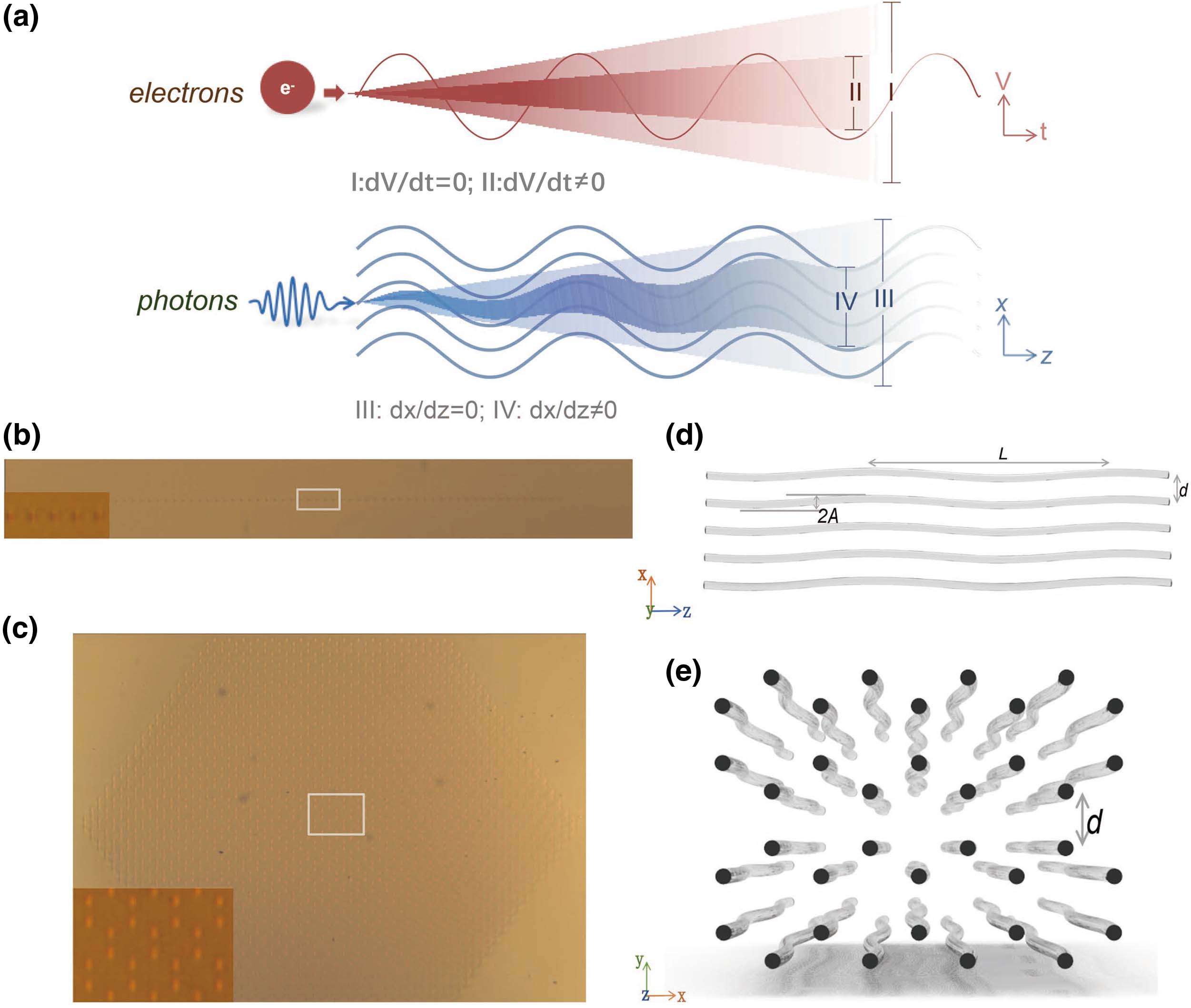
Fig. 1. The schematic of dynamic localization in a photonic lattice. (a) The suppressed evolution wave packet for electrons in an AC electric field and an analog of suppressed evolution wave packet for photons in a sinusoidally curved photonic lattice. Cross section of (b) a one-dimensional waveguide array and (c) a two-dimensional hexagonal waveguide array. The detailed schematic for the part inside the white rectangles in (b) and (c) is shown in (d) and (e), respectively, where each waveguide is modulated into sinusoidal bending on the x–z plane.

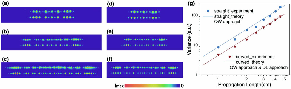
Fig. 2. Photon evolution and transport properties for one-dimensional arrays. Probability distributions for (a)–(c) straight and (d)–(f) sinusoidally curved arrays. Each scenario has an experimental pattern shown in the upper row and a theoretical pattern using the quantum walk approach shown in the row below. The propagation lengths are 1.5 cm for (a) and (d), 3 cm for (b) and (e), and 4.5 cm for (c) and (f). (g) The variance against propagation length from the experimental pattern, theoretical quantum walk approach, and theoretical dynamic localization approach. Details about error bars on experimental results are given in Appendix C.

Fig. 3. Photon evolution and transport properties for hexagonal two-dimensional arrays. (a) Schematic of the cross section of a hexagonal two-dimensional array with the effective anisotropic coupling coefficients and effective sinusoidal amplitude along different directions marked in the figure. Probability distributions for (b) straight and (c) sinusoidally curved hexagonal two-dimensional waveguide arrays. The propagation lengths for both (b) and (c) are 2.5 cm. (d) The variance against propagation length from the experimental pattern and theoretical quantum walk approach. Details about error bars on experimental results are given in Appendix C.

Fig. 4. The nearly complete dynamic localization in integrated photonics. (a) Photons spread out in the 1.2-cm-long straight array, whereas, localizing in the injection site in the curved array of the same length. The straight and curved arrays have effective coupling coefficients of 0.15 and 0.02  cm−1, respectively, for photons at a wavelength of 810 nm. The set parameters for fabricating the curved array include a period L of 1.20 cm, an amplitude A of 30 μm, and waveguide spacing d of 13 μm. (b) The measured result of cross correlation and autocorrelation of the photon source and after the chip of 1.2-cm-long curved array. (c) The measured variance of a 2-cm-long straight array, and the combined array with the 1.2-cm-long curved array placed before or after the 2-cm-long straight array, named the curved–straight and straight–curved arrays, respectively. The dashed line suggests the theoretical variance for a 2-cm-long straight array. (d)–(f) The experimentally measured cross-sectional evolution patterns and the theoretical longitudinal evolution patterns (considering an effective coupling coefficient of 0.15 and 0.02  cm−1 for the straight and curved parts) for (d) the pure straight, (e) curved–straight, and (f) straight–curved arrays.

Fig. 5. Different paths for evolution in the horizontal direction in a hexagonal two-dimensional array. The evolution Paths I–III are shown by arrows in orange, green, and blue, respectively.