Experimental quantum simulation of dynamic localization on curved photonic lattices

Hao Tang; Tian-Yu Wang; Zi-Yu Shi; Zhen Feng; Yao Wang; Xiao-Wen Shang; Jun Gao; Zhi-Qiang Jiao; Zhan-Ming Li; Yi-Jun Chang; Wen-Hao Zhou; Yong-Heng Lu; Yi-Lin Yang; Ruo-Jing Ren; Lu-Feng Qiao; Xian-Min Jin

doi:10.1364/PRJ.439637

Abstract

Dynamic localization, which originates from the phenomena of particle evolution suppression under an externally applied AC electric field, has been simulated by suppressed light evolution in periodically curved photonic arrays. However, experimental studies on their quantitative dynamic transport properties and application for quantum information processing are rare. Here we fabricate one-dimensional and hexagonal two-dimensional arrays both with sinusoidal curvatures. We successfully observe the suppressed single-photon evolution patterns, and for the first time, to the best of our knowledge, measure the variances to study their transport properties. For one-dimensional arrays, the measured variances match both the analytical electric-field calculation and the quantum walk Hamiltonian engineering approach. For hexagonal arrays as anisotropic effective couplings in four directions are mutually dependent, the analytical approach suffers, whereas quantum walk conveniently incorporates all anisotropic coupling coefficients in the Hamiltonian and solves its exponential as a whole, yielding consistent variances with our experimental results. Furthermore, we implement a nearly complete localization to show that it can preserve both the initial injection and the wave packet after some evolution, acting as a memory of a flexible time scale in integrated photonics. We demonstrate a useful quantum simulation of dynamic localization for studying their anisotropic transport properties and a promising application of dynamic localization as a building block for quantum information processing in integrated photonics.

1. INTRODUCTION

Quantum walks, the evolution with quantum coherence and ballistic transport properties [1 –3], have in recent years become a remarkably versatile tool for quantum simulation of various physics and multidisciplinary problems [4 –13]. Quantum simulation is to use the Hamiltonian matrix formed by a quantum system to simulate the Hamiltonian matrix in other target systems [4,5]. Manipulation on the quantum walk can be used to simulate quantum open systems [7 –9,14,15], graph search [16], diffusive transport in non-Hermitian lattices [10], the Anderson localization [11,12], and topologically protected bound states [13], etc., rendering highly diverse transport properties. Now, quantum walks have been successfully demonstrated in various physical systems, such as trapped ions [17], a nuclear magnetic resonator [18], superconducting qubits [19], and photons [20 –24], and the scale has risen to two-dimensional spaces with up to thousands of evolution paths in integrated photonics [25 –27]. Therefore, the power for quantum simulation using quantum walk experiments continues growing.

Dynamic localization is a physics term first introduced to describe the suppression of particle evolution under an externally applied AC electric field [28]. For cold atoms [29], Bose–Einstein condensates [30], and photons [31], such phenomena of narrowed evolution wave packets have also been observed where the applied AC electric field is mimicked by either the shaken force in the optical lattice [30] or the periodical curvature in the photonic waveguide [31]. The suppressed evolution wave packets for electrons in an AC electric field and an analog for photons in a sinusoidally curved photonic lattice are illustrated in Fig. 1(a). Dynamic localization under certain lattice/waveguide geometry could even limit the evolution completely, i.e., particles localize in the original single waveguide in the one-dimensional waveguide array [30], or evolve in only one dimension of the two-dimensional waveguide array [32].

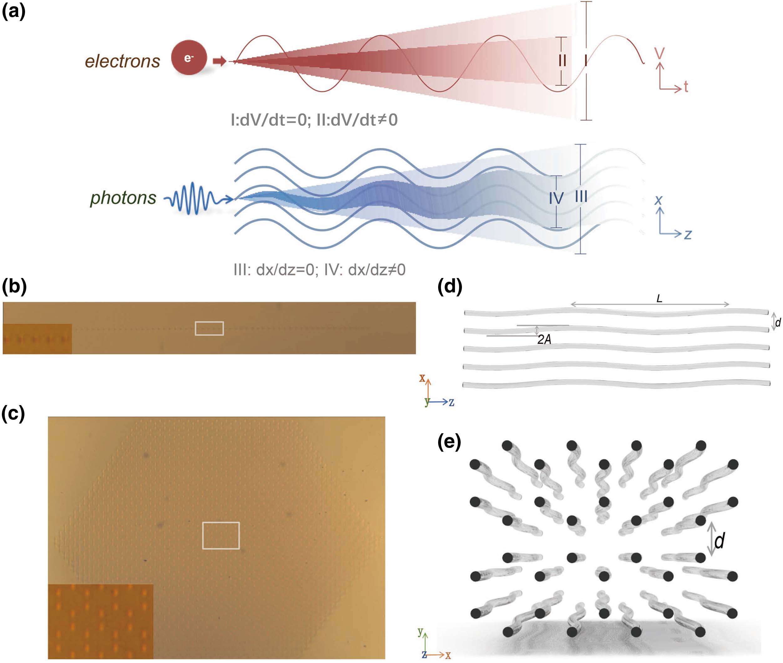
Figure 1.The schematic of dynamic localization in a photonic lattice. (a) The suppressed evolution wave packet for electrons in an AC electric field and an analog of suppressed evolution wave packet for photons in a sinusoidally curved photonic lattice. Cross section of (b) a one-dimensional waveguide array and (c) a two-dimensional hexagonal waveguide array. The detailed schematic for the part inside the white rectangles in (b) and (c) is shown in (d) and (e), respectively, where each waveguide is modulated into sinusoidal bending on the $x - z$ plane.

The name of dynamic localization is reminiscent of another kind of localization, e.g., Anderson localization [33], but their principles differ dramatically. The former is related to the rotating vectors induced by the applied field [28,34] rather than the diffusive scattering for the latter [33]. Whereas, Anderson localization has been studied extensively in quantum simulation [11,12], simulating dynamic localization in different quantum systems remains as a simple demonstration, and its time-dependent transport properties have never been experimentally reported, partially due to previous challenges in generating lots of paths for long-time evolution. However, the transport property does matter for wide applications of dynamic localization, ranging from the anisotropy in electron mobility [34], the evolution in spin systems [35], and atom trapping in a two-level system [36], etc., to the generation of anisotropic transport for any originally isotropic material [28]. Therefore, it is of great significance to study the transport properties in dynamic localization.

Sign up for Photonics Research TOC. Get the latest issue of Photonics Research delivered right to you！Sign up now

In this paper, we report on the experimental demonstration of dynamic localization employing quantum walks on both one-dimensional and hexagonal two-dimensional arrays by injecting heralded single photons into the sinusoidally curved photonic waveguides. We for the first time, to our knowledge, observe that the suppressed evolution wave packet shows ballistic transport behavior, suggesting that photonic evolution with dynamic localization still shows the nature of quantum walks. The experimental results for the one-dimensional scenario agree well with theoretical predictions by both the analytical electric-field calculation and the quantum walk approach. However, for hexagonal two-dimensional scenarios as the anisotropic effective couplings in all directions are not orthogonal and are mutually dependent, the analytical approach is severely challenging. On the other hand, we use the two-dimensional quantum walk approach to efficiently work out consistent transport properties with experiments by considering the anisotropic coupling coefficients in its Hamiltonian and calculating the probalility distribution. Therefore, we demonstrate quantum walks as a very useful tool to simulate the anisotropic transport in dynamic localization. Furthermore, we utilize a nearly complete dynamic localization to preserve the evolution packet that can create a flexible length of memory in the evolution path, demonstrating a promising application of dynamic localization for quantum information processing in integrated photonics.

2. MAIN

In our paper, we consider two array structures, the one-dimensional and hexagonal two-dimensional array with their cross sections shown in Figs. 1(b) and 1(c), respectively. For each structure, two categories of waveguides are prepared, the straight ones and the sinusoidally curved ones. The sinusoidal curvature, although not very clearly seen in the cross section due to its marginal size, does exist along the propagation direction $z$ and bends horizontally on the $x - z$ plane. The curvature has a period $L$ of 2 cm and an amplitude $A$ of 14.4 μm in the array with a waveguide spacing $d$ of 15 μm as shown in Figs. 1(d) and 1(e).

The dynamic localization of a charged particle moving under the sinusoidal driving field [28] and the quantum analogy in the photonic lattice [31,37,38] [Fig. 1(a)] can both be described by a Schrödinger equation with a periodic curvature along the evolution direction. By applying a discrete model of the tight-binding approximation, the total field is decomposed into a superposition of weakly overlapping modes of the individual waveguides and becomes a common coupled mode theory [37 –39], which can be solved to get the probability distribution, and suggest the suppressed evolution packets when the AC field or lattice curvature exists. A derivation from the discrete-time Schrödinger equation to the differential wave equation is given in Appendix A.

Quantum walks can also be derived from such a discrete-time Schrödinger equation, but they are more commonly discussed directly in the context of the Hamiltonian matrix and coupling coefficients. From a quantum walk perspective, the wavefunction that evolves from an initial wavefunction satifies: $| Ψ (z) ⟩ = e^{- i H z} | Ψ (0) ⟩$ , and the evolution profile can be obtained by the matrix exponential method when the Hamiltonian $H$ is known [25]. For photons propagating through coupled waveguide arrays, $H$ can be described as $H = \sum_{i}^{N} β_{i} a_{i}^{†} a_{i} + \sum_{i \neq j}^{N} C_{i, j} a_{i}^{†} a_{j},$ (1)where $β_{i}$ is a propagating constant in waveguide $i$ and $C_{i, j}$ is the coupling coefficient between waveguides $i$ and $j$ .

For the sinusoidally curved array, the curvature causes the suppressed evolution packets that are equivalent to the reducing of the coupling coefficient. The effective coupling coefficient becomes [38] $C_{eff} = C_{0} J_{0} (\frac{2 π ω A}{L}),$ (2)where $C_{0}$ is the original coupling coefficient before adding curvature to the straight waveguide. $J_{0}$ is the Bessel function of the first kind, and $ω = 2 π n_{0} d / λ$ , where $n_{0} = 1.503$ is the substrate refractive index, and $λ = 780 nm$ is the wavelength of the input photon source. $d$ , $A$ , and $L$ are the curvature indices marked in Fig. 1(b). Replacing $C$ with $C_{eff}$ in Eq. (1) enables the inclusion of the curvature-induced transport effect in the quantum walk approach. Some explanation on deriving $C_{eff}$ can be found in Appendix B.

In the experiment, we then inject a vertically polarized 780-nm heralded single-photon source (see Methods section) into the central waveguide of each array from one end of the photonic chip and capture the evolution pattern at the other end using an intensified charge-coupled device (ICCD) camera. The measured light intensity patterns represent the probability distribution after certain propagation lengths. The evolution result from the theoretical quantum walk approach with $C_{eff}$ and the experimental measurement are both plotted in Figs. 2(a)–2(f). Meanwhile, the variance as a common parameter to measure the transport properties is defined by $σ {(z)}^{2} = \frac{\sum_{i = 1}^{N} {(Δ l_{i})}^{2} P_{i} (z)}{\sum_{i = 1}^{N} P_{i} (z)},$ (3)where $P_{i} (z)$ is the probability of the walker at waveguide $i$ at propagation length $z$ and $Δ l_{i}$ is the normalized distance from the original waveguide. In the experiment, we have made lattice sizes much larger than the evolution patterns to avoid the boundary effects that may affect the variance estimation. The variance as shown in Fig. 2(g) has a value for the curved array much lower than that for the straight array due to the suppressed $C_{eff}$ , but a ballistic feature appears in both the straight and the curved arrays. This proves that despite a smaller coupling coefficient, the evolution in the periodically curved lattice still obeys a quantum walk when the imaginary part of $C$ that represents loss caused by the small curvature [10] is almost negligible.

Figure 2.Photon evolution and transport properties for one-dimensional arrays. Probability distributions for (a)–(c) straight and (d)–(f) sinusoidally curved arrays. Each scenario has an experimental pattern shown in the upper row and a theoretical pattern using the quantum walk approach shown in the row below. The propagation lengths are 1.5 cm for (a) and (d), 3 cm for (b) and (e), and 4.5 cm for (c) and (f). (g) The variance against propagation length from the experimental pattern, theoretical quantum walk approach, and theoretical dynamic localization approach. Details about error bars on experimental results are given in Appendix C.

Meanwhile, the variance in the one-dimensional lattice has already been derived for dynamic localization [28,34], which is simply given by $σ {(z)}^{2} = σ_{0} {(z)}^{2} J_{0}^{2} (\frac{2 π ω A}{L}),$ (4)where $σ_{0}^{2}$ is the variance for the corresponding straight array. The dynamic localization approach analytically solves the variance as a function of the Bessel terms that represent the curvature profile, and this gives a value of variance that is highly consistent with those from the quantum walk approach and the experimental approach as shown in Fig. 2(g). This is not a surprise because both the quantum walk approach and the dynamic localization approach derive from the same discrete Schrödinger model but just approach differently: the former considers the curvature in the modified coupling coefficients in its Hamiltonian and gets the variance from the calculated probability distribution, and the latter tries to give an analytic solution of the variance that takes the curvature function into consideration.

When the dimension of photonic waveguide arrays increases to two, higher complexities are inevitably incurred. $A$ in Eq. (2) should be replaced by $A_{m}$ , the effective amplitude. $A_{m}$ can be calculated as $A \cos θ$ , where $θ$ is the angle between the coupling direction and the horizontal curvature direction. Therefore, $C_{eff}$ allows for the anisotropic transport effect in the quantum walk approach. In Fig. 3(a), $h$ , $h 30$ , $h 60$ , and $v$ represent the four possible directions of the two coupled waveguides, namely, horizontal, 30° for a horizontal line, 60° for a horizontal line, and vertical, corresponding to an $A_{m}$ of $A \cos 0 °$ , $A \cos 30 °$ , $A \cos 60 °$ , and $A \cos 90 °$ , respectively. Besides, there are three types of waveguide spacings to be considered, namely, $d$ , $\sqrt{3} d$ , and $2 d$ . Taking both direction and waveguide spacing into consideration, this gives totally six different scenarios for effective coupling coefficients as have been marked in Fig. 3(a).

Figure 3.Photon evolution and transport properties for hexagonal two-dimensional arrays. (a) Schematic of the cross section of a hexagonal two-dimensional array with the effective anisotropic coupling coefficients and effective sinusoidal amplitude along different directions marked in the figure. Probability distributions for (b) straight and (c) sinusoidally curved hexagonal two-dimensional waveguide arrays. The propagation lengths for both (b) and (c) are 2.5 cm. (d) The variance against propagation length from the experimental pattern and theoretical quantum walk approach. Details about error bars on experimental results are given in Appendix C.

Now, in the hexagonal two-dimensional scenarios, the analytical dynamic localization approach suffers. Transferring from the one-dimensional analytics [28] to multidimensional transport requires the independent coupling in different directions [34]. However, this is not possible in the hexagonal structure shown in Fig. 3(a). The photon evolution is continuously varying among $h$ , $h 30$ , $h 60$ , and $v$ directions, which makes the transport in each direction never independent at any time. More explanation on why it is almost impossible to give the analytical solution to variance for the hexagonal two-dimensional scenario is given in Appendix D. On the other hand, using the quantum walk approach, we put the anisotropic coupling coefficient into the Hamiltonian and conveniently generate the two-dimensional evolution pattern using the exactly same matrix exponential method as in the one-dimensional scenario.

As demonstrated in Fig. 3(b), the experimental two-dimensional evolution pattern for the straight array is almost isotropic, but the evolution in the curved array in Fig. 3(c) is faster vertically than horizontally, making a rectangular shape of the pattern. The variance in different directions is presented in Fig. 3(d), suggesting the ballistic relationship for the evolution in both straight and curved arrays. It also demonstrates that the vertical variance always exceeds the horizontal variance for the curved arrays, which can be associated with the exemption of $C_{eff}$ modulation in the vertical direction because $A_{mv} = A \cos 90 ° = 0$ and $J_{0} (0) = 1$ . However, it is worth noting that the vertical variances in the curved arrays remain lower than those in the straight arrays, owing to the complexity of waveguide coupling in two-dimensional arrays. The couplings in $h 30$ and $h 60$ directions are both to some extent suppressed, and although they did not point to the vertical direction directly, the evolution through these restrained paths inevitably influences the vertical pattern and variance. The quantum walk approach does not have to separately treat each directed coupling but calculates the profile as a whole, and this solves the evolution puzzle, which is, otherwise, overcomplicated using the analytical dynamic localization approach.

Furthermore, we demonstrate a potential application of dynamic localization for creating a memory function in quantum information processing. We prepare a one-dimensional array with specially manipulated parameters that make $C_{eff}$ in Eq. (2) drop to nearly zero. As shown in Fig. 4(a), photons spread out in the straight array of 1.2 cm, whereas, almost localizing in the injection site in the curved array of the same length. For this chip of the 1.2-cm-long curved array, we measure the cross correlation and autocorrelation of the photon source before and after the chip [in Fig. 4(b)], both obtaining a Cauchy–Schwarz inequality violation by 1303 and 125 standard deviations, respectively. (See the details in Appendix E.) This demonstrates that dynamic localization still well preserves the nonclassical property in the integrated photonics. We use such a curved array as a building block to place it before and after a 2-cm-long straight array. Comparing with the evolution pattern for the straight array [Fig. 4(d)], the curved–straight array [Fig. 4(e)] well preserves the initial state in the input site. More interestingly, we show that the straight–curved array can preserve the spreadout wave packet as well [Fig. 4(f)]. Both the curved–straight and the straight–curved arrays yield similar variance with the straight-only array [Fig. 4(c)]. This is very meaningful, especially for the straight–curved scenario, which is rarely investigated since this shows that if we want a quantum walk to pause for a flexible length of time, we can just smoothly connect the straight array with a well-designed curved array that leads to dynamic localization. This can perform a very practical memory function in integrated photonics.

Figure 4.The nearly complete dynamic localization in integrated photonics. (a) Photons spread out in the 1.2-cm-long straight array, whereas, localizing in the injection site in the curved array of the same length. The straight and curved arrays have effective coupling coefficients of 0.15 and $0.02 {cm}^{- 1}$ , respectively, for photons at a wavelength of 810 nm. The set parameters for fabricating the curved array include a period $L$ of 1.20 cm, an amplitude $A$ of 30 μm, and waveguide spacing $d$ of 13 μm. (b) The measured result of cross correlation and autocorrelation of the photon source and after the chip of 1.2-cm-long curved array. (c) The measured variance of a 2-cm-long straight array, and the combined array with the 1.2-cm-long curved array placed before or after the 2-cm-long straight array, named the curved–straight and straight–curved arrays, respectively. The dashed line suggests the theoretical variance for a 2-cm-long straight array. (d)–(f) The experimentally measured cross-sectional evolution patterns and the theoretical longitudinal evolution patterns (considering an effective coupling coefficient of 0.15 and $0.02 {cm}^{- 1}$ for the straight and curved parts) for (d) the pure straight, (e) curved–straight, and (f) straight–curved arrays.

3. DISCUSSION

In conclusion, we investigated the experimental single-photon distribution in sinusoidally curved arrays and measured the variances that suggested ballistic transport properties. We considered two theoretical approaches to analyzing variances. The first was an analytical solution as a function of the curvature parameters, which had already been derived for dynamic localization in the one-dimensional array. The other was to treat the evolution as a quantum walk process. It incorporated all anisotropic coupling coefficients in its Hamiltonian and gave the probability distribution by solving the Hamiltonian exponential as a whole, and the variance can then be numerically calculated from the probability distribution.

It turned out that both approaches worked well for the evolution in the one-dimensional array. However, for the hexagonal two-dimensional array because the anisotropic effective coupling in four directions was mutually dependent, it was infeasible to apply the analytical dynamic localization approach. On the other hand, the quantum walk approach conveniently and efficiently gave the variances that matched our experimental results very well. We had, thus, demonstrated a promising application of two-dimensional quantum walks in simulating dynamic localization. This was meaningful for quantum materials as it studied the prevalent anisotropic transport properties in materials.

From this paper, we also saw that the effective coupling coefficients caused by dynamic localization can be very flexibly manipulated by experimentally tuning different parameters, namely, the curvature amplitude $A$ , the longitudinal period $L$ , the waveguide spacing $d$ , the refractive index $n$ , and the wavelength $λ$ . In recent years, there was a growing number of promising studies on quantum information sciences using integrated photonics [40 –45]. We have demonstrated a nearly complete dynamic localization to create a memory function in integrated photonics, and it can be widely used to experimentally manipulate coupling coefficients for more Hamiltonian engineering tasks.

Furthermore, this paper demonstrated an inspiring example of mapping certain wave equations to quantum walks that can be experimentally implemented on a photonic chip. This approach can be well applied to simulating plenty more wave equations, for instance, the Aubry–André–Harper model [46], the Su–Schrieffer–Heeger model [43], and other models in topological photonics and condensed-matter physics. Our strong capacity in achieving a large-scale three-dimensional photonic chip demonstrated a promising potential for quantum simulation in a highly diverse regime.

4. METHODS

Waveguide preparation. Waveguide arrays were prepared by directing a femtosecond laser (10-W, 1026-nm, 290-fs pulse duration, 1-MHz repetition rate, and 513-nm working frequency) into a spatial light modulator (SLM) to create burst trains onto a borosilicate substrate with a $50 \times$ objective lens (numerical aperture: 0.55) at a constant velocity of 10 mm/s. Power and SLM compensation were processed to ensure the waveguides were uniform and depth independent [25,26].

Heralded single-photon preparation and single-photon-level imaging. We used a frequency doubled 390-nm-fs laser pump and a 2-mm-thick $β$ -barium borate crystal to generate degenerate 780-nm photon pairs via a type-II spontaneous parametric downconversion process in the beamlike scheme. The photons were then filtered by a 3-nm bandpass filter and guided to the photonic chip [47,48]. We injected the vertically polarized photon into the center waveguide in the photonic chip, whereas the horizontally polarized photon was connected to a single-photon detector that set a trigger for heralding the vertically polarized photons with the ICCD camera with a time slot of 10 ns. Without the external trigger, the measured patterns came from the thermal-state light rather than single photons. The ICCD camera captured each evolution pattern with a certain evolution length after accumulating in the external mode for 1–1.5 h.

Acquisition of variance for probability distribution. When collecting the data from experiments, we obtained the corresponding advanced scientific computer II file, which was essentially a matrix of pixels. We created a “mask” that contained the coordinate of the circle center and the radius in pixels for each waveguide and summed up the light intensity for all the pixels within each circle using MATLAB. The normalized proportion of light intensity for each circle represented the probability at the corresponding waveguide.

Acknowledgment

Acknowledgment. This research was supported by the National Key R&D Program of China, National Natural Science Foundation of China, Science and Technology Commission of Shanghai Municipality, and Shanghai Municipal Education Commission. X.-M.J. acknowledges additional support from a Shanghai talent program and support from Zhiyuan Innovative Research Center of Shanghai Jiao Tong University.

X.-M.J. conceived and supervised the project. H.T. designed the experiment. Z.F. prepared the samples. H.T., Z.-Y.S., T.-Y.W., and Z.F. conducted the experiment presented in Figs. 2 and 3. H.T., T.-Y.W., Y.-J.C, and Y.-L.Y conducted the new experiment on the nearly complete dynamic localization presented in Fig. 4. H.T., X.-W.S., Y.W., J.G., and Y.-H.L. carried out theoretical analysis. Z.-Q.J., Z.-M.L., and R.-J.R. implemented the single-photon setup. H.T., T.-Y.W., Z.-Y.S., X.-W.S., W.-H.Z., and L.-F.Q. processed the data. H.T. wrote the paper with input from all the other authors.

APPENDIX A: DERIVE THE COUPLED MODE DERIVATIVE EQUATION FROM THE DISCRETE-TIME SCHR?DINGER EQUATION

z

E (x, z)

i \frac{\partial Ψ_{m}}{\partial z} = - C (Ψ_{m + 1} + Ψ_{m - 1}) + ω {\ddot{x}}_{d} (z) Ψ_{m},

t

x_{d} (z)

APPENDIX B: OBTAIN THE EFFECTIVE COUPLING COEFFICIENT

C_{eff}

x_{d} (z)

A

APPENDIX C: DETAILS ABOUT THE ERROR BARS FOR EXPERIMENTAL RESULTS

In this paper, we performed one experiment for each dot shown in Figs. 2 (g) and 3 (d). The main source for the error may lie in the evaluation of photon counts as the background noise, which would influence the characterizing of the light intensity of each waveguide mode and, hence, the probability distribution and variance. This is because the single-photon experiment renders each picture via 1- to 2-h accumulation of single photons and is sensitive to multiple noise sources throughout the photonic setup. From the raw data of one experiment, for instance, whereas the brightest pixel may have a count of 159,788, the pixels for background noise have counts of above 96,000, so a proper choice of the background noise count matters.

1024 \times 1024

As the original Figs. 2 (g) and 3 (d) already contain lots of content, it may not be very clear if further adding error bars into each dot represents a mean value of the variances. Therefore, we separately provide values of error bars for the one- and two-dimensional lattices in Tables 1 and 2, respectively. The unit is consistent with the mean values of the variances in Figs. 2 (g) and 3 (d). Table 1.

Error Bars for the Variances from Experimental Results in Fig. 2(g) for One-Dimensional Lattices of Different Propagation Lengths

$z$ (cm)	Straight lattice	Curved lattice
1.0	0.0247	0.2696
1.5	0.2232	0.4490
2.0	0.3183	0.2616
2.5	0.0506	0.1722
3.0	0.0119	1.0637
3.5	0.2134	2.7872
4.0	0.0648	0.1983
4.5	9.6076	0.3308

Table 2.

Error Bars for the Variances from Experimental Results in Fig. 3(d) for Two-Dimensional Lattices of Different Propagation Lengths

$z$ (cm)	Straight_ $h$	Straight_ $v$	Curved_ $h$	Curved_ $v$
1.0	0.2093	0.1869	0.4089	0.2664
1.5	2.0750	0.3057	2.4446	1.5323
2.0	3.0069	1.0274	3.4003	1.9128
2.5	0.1039	0.1272	2.1075	0.8895
3.0	0.3904	0.1215	1.6214	0.4763
3.5	1.2273	0.3511	2.0750	0.3057

APPENDIX D: EXPLAIN WHY IT IS DIFFICULT TO EXTEND THE ANALYTICAL APPROACH TO HEXAGONAL TWO-DIMENSIONAL SCENARIOS

σ {(z)}^{2} = 2 C^{2} [u^{2} (z) + v^{2} (z)],

η (z)

σ_{0} {(z)}^{2} = 2 C^{2} z^{2}

h

h

d

Figure 5.Different paths for evolution in the horizontal direction in a hexagonal two-dimensional array. The evolution Paths I–III are shown by arrows in orange, green, and blue, respectively.

h 30

h

APPENDIX E: MEASUREMENTS OF CROSS CORRELATION AND AUTOCORRELATION

g_{e c}^{(2)}

{(g_{e c}^{(2)})}^{2} \leq g_{e e}^{(2)} g_{c c}^{(2)} .

\frac{{(g_{e c}^{(2)})}^{2} - g_{e e}^{(2)} g_{c c}^{(2)}}{δ_{total}},

g_{e c}^{(2)}

References

[1] Y. Aharonov, L. Davidovich, N. Zagury. Quantum random walks. Phys. Rev. A, 48, 1687-1690(1993).

[2] A. M. Childs, E. Farhi, S. Gutmann. An example of the difference between quantum and classical random walks. Quantum Inf. Process, 1, 35-43(2002).

[3] O. Mülken, A. Blumen. Continuous-time quantum walks: models for coherent transport on complex networks. Phys. Rep., 502, 37-87(2011).

[4] I. Buluta, F. Nori. Quantum simulators. Science, 326, 108-111(2009).

[5] I. M. Georgescu, S. Ashhab, F. Nori. Quantum simulation. Rev. Mod. Phys., 86, 153-185(2014).

[6] A. Aspuru-Guzik, P. Walther. Photonic quantum simulators. Nat. Phys., 8, 285-291(2012).

[7] J. D. Whitfield, C. A. -RosarioRodríguez, A. Aspuru-Guzik. Quantum stochastic walks: a generalization of classical random walks and quantum walks. Phys. Rev. A, 81, 022323(2010).

[8] D. N. Biggerstaff, R. Heilmann, A. A. Zecevik, M. Gräfe, M. A. Broome, A. Fedrizzi, I. Kassal. Enhancing coherent transport in a photonic network using controllable decoherence. Nat. Commun., 7, 11208(2016).

[9] H. Tang, Z. Feng, Y. H. Wang, P. C. Lai, C. Y. Wang, Z. Y. Ye, C. K. Wang, Z. Y. Shi, T. Y. Wang, Y. Chen, J. Gao, X.-M. Jin. Experimental quantum stochastic walks simulating associative memory of Hopfield neural networks. Phys. Rev. Appl., 11, 024020(2019).

[10] T. Eichelkraut, R. Heilmann, S. Weimann, S. Stützer, F. Dreisow, D. N. Christodoulides, S. Nolte, A. Szameit. Mobility transition from ballistic to diffusive transport in non-Hermitian lattices. Nat. Commun., 4, 143604(2013).

[11] Y. Lahini, A. Avidan, F. Pozzi, M. Sorel, R. Morandotti, D. N. Christodoulides, Y. Silberberg. Anderson localization and nonlinearity in one-dimensional disordered photonic lattices. Phys. Rev. Lett., 100, 013906(2008).

[12] A. Schreiber, K. N. Cassemiro, V. Potoček, A. Gábris, I. Jex, C. Silberhorn. Decoherence and disorder in quantum walks: from ballistic spread to localization. Phys. Rev. Lett., 106, 180403(2011).

[13] T. Kitagawa, M. A. Broome, A. Fedrizzi, M. S. Rudner, E. Berg, I. Kassal, A. Aspuruguzik, E. Demler, A. G. White. Observation of topologically protected bound states in photonic quantum walks. Nat. Commun., 3, 882(2012).

[14] L. Banchi, D. Burgarth, M. J. Kastoryano. Driven quantum dynamics: will it blend?. Phys. Rev. X, 7, 041015(2017).

[15] H. Tang, L. Banchi, T. Y. Wang, X. W. Shang, X. Tan, W. H. Zhou, Z. Feng, A. Pal, H. Li, C. Q. Hu, M. S. Kim, X.-M. Jin. Generating Haar-uniform randomness using stochastic quantum walks on a photonic chip. Phys. Rev. Lett., 128, 050503(2022).

[16] S. D. Berry, J. B. Wang. Quantum-walk-based search and centrality. Phys. Rev. A, 82, 042333(2010).

[17] H. Schmitz, R. Matjeschk, C. Schneider, J. Glueckert, M. Enderlein, T. Huber, T. Schaetz. Quantum walk of a trapped ion in phase space. Phys. Rev. Lett., 103, 090504(2009).

[18] J. Du, H. Li, X. Xu, M. Shi, J. Wu, X. Zhou, R. Han. Experimental implementation of the quantum random-walk algorithm. Phys. Rev. A, 67, 042316(2003).

[19] M. Gong, S. Y. Wang, C. Zha. Quantum walks on a programmable two-dimensional 62-qubit superconducting processor. Science, 372, 948-952(2021).

[20] H. B. Perets, Y. Lahini, F. Pozzi, M. Sorel, R. Morandotti, Y. Silberberg. Realization of quantum walks with negligible decoherence in waveguide lattices. Phys. Rev. Lett., 100, 170506(2008).

[21] A. Peruzzo, M. Lobino, J. C. F. Matthews, N. Matsuda, A. Politi, K. Poulios, X.-Q. Zhou, Y. Lahini, N. Ismaili, K. Worhoff, Y. Bromberg, Y. Silberberg, M. G. Thompson, J. L. O’Brien. Quantum walks of correlated photons. Science, 329, 1500-1503(2010).

[22] A. Schreiber, A. Gábris, P. P. Rohde, K. Laiho, M. Štefaňák, V. Potoček, C. Hamilton, I. Jex, C. Silberhorn. A 2D quantum walk simulation of two-particle dynamics. Science, 336, 55-58(2012).

[23] Y. C. Jeong, C. Di Franco, H. T. Lim, M. S. Kim, Y. H. Kim. Experimental realization of a delayed-choice quantum walk. Nat. Commun., 4, 2471(2013).

[24] Z. Y. Shi, H. Tang, Z. Feng, Y. Wang, Z. M. Li, J. Gao, Y. J. Chang, T. Y. Wang, J. P. Dou, Z. Y. Zhang, Z. Q. Jiao, W. H. Zhou, X. M. Jin. Quantum fast hitting on glued trees mapped on a photonic chip. Optica, 7, 613-618(2020).

[25] H. Tang, X. F. Lin, Z. Feng, J. Y. Chen, J. Gao, K. Sun, C. Y. Wang, P. C. Lai, X. Y. Xu, Y. Wang, L. F. Qiao, A. L. Yang, X. M. Jin. Experimental two-dimensional quantum walk on a photonic chip. Sci. Adv., 4, eaat3174(2018).

[26] H. Tang, C. Di Franco, Z. Y. Shi, T. S. He, Z. Feng, J. Gao, Z. M. Li, Z. Q. Jiao, T. Y. Wang, M. S. Kim, X. M. Jin. Experimental quantum fast hitting on hexagonal graphs. Nat. Photonics, 12, 754-758(2018).

[27] X. Y. Xu, X. W. Wang, D. Y. Chen, C. M. Smith, X.-M. Jin. Quantum transport in fractal networks. Nat. Photonics, 15, 703-710(2021).

[28] D. H. Dunlap, V. M. Kenkre. Dynamic localization of a charged particle moving under the influence of an electric field. Phys. Rev. B, 34, 3625-3633(1986).

[29] K. W. Madison, M. C. Fischer, R. B. Diener, Q. Niu, M. G. Raizen. Dynamical Bloch band suppression in an optical lattice. Phys. Rev. Lett., 81, 5093-5096(1998).

[30] A. Eckardt, M. Holthaus, H. Lignier, A. Zenesini, D. Ciampini, O. Morsch, E. Arimondo. Exploring dynamic localization with a Bose-Einstein condensate. Phys. Rev. A, 79, 013611(2009).

[31] S. Longhi, M. Marangoni, M. Lobino, R. Ramponi, P. Laporta, E. Cianci, V. Foglietti. Observation of dynamic localization in periodically curved waveguide arrays. Phys. Rev. Lett., 96, 243901(2006).

[32] A. Szameit, I. L. Garanovich, M. Heinrich, A. A. Sukhorukov, F. Dreisow, T. Pertsch, S. Nolte, A. Tünnermann, Y. S. Kivshar. Polychromatic dynamic localization in curved photonic lattices. Nat. Phys., 5, 271-275(2009).

[33] E. Abrahams, P. W. Anderson, D. C. Licciardello, T. V. Ramakrishnan. Scaling theory of localization: absence of quantum diffusion in two dimensions. Phys. Rev. Lett., 42, 673-676(1979).

[34] V. M. Kenkre, S. Raghavan. Dynamic localization and related resonance phenomena. J. Opt. B, 2, 686-693(2000).

[35] S. Raghavan, V. M. Kenkre, A. R. Bishop. Dynamic localization in spin systems. Phys. Rev. B, 61, 5864-5867(2000).

[36] G. S. Agarwal, W. Harshawardhan. Realization of trapping in a two-level system with frequency-modulated fields. Phys. Rev. A, 50, R4465-R4467(1994).

[37] S. Longhi. Self-imaging and modulational instability in an array of periodically curved waveguides. Opt. Lett., 30, 2137-2139(2005).

[38] I. L. Garanovich, S. Longhi, A. A. Sukhorukov, Y. S. Kivshar. Light propagation and localization in modulated photonic lattices and waveguides. Phys. Rep., 518, 1-79(2009).

[39] A. A. Sukhorukov, Y. S. Kivshar. Generation and stability of discrete gap solitons. Opt. Lett., 28, 2345-2347(2003).

[40] Y. Chen, J. Gao, Z. Q. Jiao, K. Sun, L. F. Qiao, H. Tang, X. F. Lin, X. M. Jin. Mapping twisted light into and out of a photonic chip. Phys. Rev. Lett., 121, 233602(2018).

[41] Y. Wang, J. Gao, X. L. Pang, Z. Q. Jiao, H. Tang, Y. Chen, L. F. Qiao, Z. W. Gao, J. P. Dou, A. L. Yang, X. M. Jin. Experimental parity-induced thermalization gap in disordered ring lattices. Phys. Rev. Lett., 122, 013903(2019).

[42] Z. Feng, Z. W. Gao, L. A. Wu, H. Tang, K. Sun, C. Q. Hu, Y. Wang, Z. M. Li, X. W. Wang, Y. Chen, E. Z. Zhang, Z. Q. Jiao, X. Y. Xu, J. Gao, A. L. Yang, X. M. Jin. Photonic Newton’s cradle for remote energy transport. Phys. Rev. Appl., 11, 044009(2019).

[43] Y. Wang, Y. H. Lu, F. Mei, J. Gao, Z. M. Li, H. Tang, S. L. Zhu, S. T. Jia, X.-M. Jin. Direct observation of topology from single-photon dynamics on a photonic chip. Phys. Rev. Lett., 122, 193903(2019).

[44] Y. Wang, Y. H. Lu, J. Gao, Y. J. Chang, R. J. Ren, Z. Q. Jiao, Z. Y. Zhang, X. M. Jin. Topologically protected polarization quantum entanglement on a photonic chip authors. Chip, 1, 100003(2022).

[45] J. Gao, X. W. Wang, W. H. Zhou, Z. Q. Jiao, R. J. Ren, Y. X. Fu, L. F. Qiao, X. Y. Xu, C. N. Zhang, X. L. Pang, H. Li, Y. Wang, X. M. Jin. Quantum advantage with membosonsampling. Chip, 1, 100007(2022).

[46] Y. Wang, Y. H. Lu, J. Gao, K. Sun, Z. Q. Jiao, H. Tang, X.-M. Jin. Quantum topological boundary states in quasi-crystal. Adv. Mater., 31, 1905624(2019).

[47] K. Sun, J. Gao, M. M. Cao, Z. Q. Jiao, Y. Liu, Z. M. Li, E. Poem, A. Eckstein, R. J. Ren, X. L. Pang, H. Tang, I. A. Walmsley, X.-M. Jin. Mapping and measuring large-scale photonic correlation with single-photon imaging. Optica, 6, 244-249(2019).

[48] Y. H. Kim. Quantum interference with beamlike type-II spontaneous parametric down-conversion. Phys. Rev. A, 68, 013804(2003).