The ability to produce multi-layered three-dimentional (3D) imagery is of utmost importance in various applications in remote sensing^[1,2] and rescue operations in surveillance and reconnaissance^[3,4]. The application scenarios include the viewing of partially obscured targets like camouflage nets through semitransparent materials such as windows, and through distributed reflective media like foliage. However, conventional two-dimentional (2D) optical imaging approaches exhibit poor performance in multi-layer scenarios with foreground clutter. This is primarily due to the lack of depth information, which prevents effective separation of the target from the foreground clutter. In recent years, active imaging methods have been proposed to tackle this challenge, including millimeter wave radar^[5,6] and Wi-Fi imaging^[7,8]. These methods leverage the inherent ability of mm-wave and Wi-Fi signals to penetrate the clutter in front of the target. Nevertheless, it is important to note that the resolution of these methods is relatively inferior compared to optical approaches. As a result, a combination of high-resolution optical imaging and active imaging methods has positioned light detection and ranging (LiDAR)^[4,9] as a compelling technology for imaging partially concealed scenarios.

Single-photon LiDAR has witnessed rapid development because it can offer high temporal resolution and high sensitivity by using time-correlated single-photon counting (TCSPC) techniques^[10–13]. The high temporal resolution permits excellent surface-to-surface resolution for 3D imaging of multi-depth scenarios^[14]. The computational imaging algorithms have witnessed remarkable progress in processing the single photon data of complex scenes efficiently^[15–17]. Moreover, photon-efficient imaging algorithms^[18–22] have shown good performance in dealing with low return signals and high background noise, which has been successfully demonstrated in several challenging scenarios including imaging through clutter^[14,23], long-range depth imaging^[24–29], non-line-of-sight imaging^[30–32], and imaging through high levels of scattering media^[33–39].

Researchers have foreseen the potential of single-photon LiDAR in imaging of camouflaged scenarios and carried out experiments. For instance, the Jigsaw airborne system demonstrated the capability of detecting hidden objects using foliage-penetrating 3D imaging^[4]. Wallace et al. reconstructed the depth profile of an object behind a wooden trellis fence using a scanning sensor^[40]. Tobin et al. presented a scanning transceiver system for imaging targets through camouflaged nets^[23]. These results employed a scanning-based single-photon LiDAR system, which requires a relatively long acquisition time. The emergence of single-photon avalanche diode (SPAD) detector arrays significantly decreases the acquisition time by collecting returned photons in a parallel way^[41–44]. Tachella et al. utilized a SPAD array to show the remarkable real-time imaging through camouflage nets using plug-and-play point cloud denoisers^[15]. However, due to technological constraints, SPAD array-based systems normally exhibit fewer pixels and lower time resolution compared to single-point scanning sensors, leading to reduced imaging resolution.

Here, we present a single-photon LiDAR system based on an InGaAs/InP SPAD detector array to capture high-resolution 3D profiles of static and moving targets concealed by double-layer camouflage nets. For static targets, we reported a sub-voxel scanning approach^[45,46] combined with a 3D deconvolution algorithm to realize high-resolution imaging. Using this approach, we experimentally demonstrated 3D imaging through camouflage netting with a 3× improvement in spatial resolution and a 7.5× improvement in depth resolution. The average signal photons per pixel (PPP) is as few as 1.73 PPP, and the acquisition time of each sub-voxel is 10 ms. For moving targets, we proposed a motion detection and compensation algorithm to mitigate the net’s obstructive effects, achieving real-time imaging of camouflaged scenes at 20 frame/s. Different from Ref. [15], our approach exploits the correlation between different frames, which can avoid the loss of photons in some pixels due to the occlusion of the camouflage nets. To verify our approach, we perform a series of experiments in daylight and night for an outdoor complex scene and test the results through glass door and camouflage nets using a single-photon LiDAR, a visible-light camera, and a mid-wave infrared (MWIR) camera.

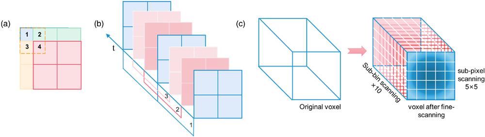
Constrained by factors such as material uniformity, circuit fabrication technology, data transmission, and cost, the format and time resolution of SPAD detector arrays are currently limited, preventing them from achieving high-resolution imaging in multi-depth scenarios. To improve the depth resolution, Rapp et al. introduced subtractive dither to the temporal quantization of TCSPC^[47], while Raghuram et al. achieved super-resolving transients by oversampled measurements^[48]. Inspired by these works, we proposed the 3D sub-voxel scanning approach and a tailored spatial-temporal photon-efficient deconvolution algorithm (see Fig. 1), which can alleviate the block effect of the foreground clutter and achieve super-resolution image reconstruction with about 1 PPP. The sub-pixel scanning method, initially employed in conventional cameras, captures a series of low-resolution images during the sub-pixel displacement process, which can be reconstructed to obtain a high-resolution image^[49]. This method has also been applied in single-photon imaging in recent years^[50]. For instance, Li et al. utilized the sub-pixel scanning approach to achieve super-resolution imaging beyond the diffraction limit over long distances^[45,46].

To achieve 3D sub-voxel scanning, we employed a piezo tip/tilt platform with a mirror and an arbitrary function generator (AFG) for sub-pixel scanning in the spatial domain and sub-bin scanning in the temporal domain, respectively. To realize sub-pixel scanning, we set the inter-pixel scanning space smaller than the size of the field of view (FoV) of one pixel. As shown in Fig. 1(a), we illustrate an inter-pixel spacing of 1/2 FoV as an example. The inter-pixel shift was performed in both the x and y directions [Fig. 1(a)]. After scanning all the pixels, a high-resolution image (320 pixel × 320 pixel) was computed by combining frames of low-resolution images (64 pixel × 64 pixel). In the temporal domain, considering that the time resolution of the time-to-digital converter (TDC) was 1 ns, the histogram bin width during the imaging process was set to 1 ns, corresponding to a depth resolution of 15 cm. To improve the depth resolution, we applied the AFG to perform sub-bin scanning with a step size of 1/10 of the bin width between the laser and the SPAD array [as shown in Fig. 1(b), an example of 1/3 sub-bin scanning]. This enabled us to obtain 10 frames with low temporal resolution, which could then be processed to derive an image with high temporal resolution.

To cooperate with our 3D sub-voxel scanning approach, we develop a spatial-temporal photon-efficient deconvolutional algorithm to compute the high-resolution image from the sub-voxel scanning data with low signal levels at ∼1PPP. The algorithm takes the sub-voxel fine scanning process into account in the forward model and combines a 3D deconvolution method to retrieve the sub-voxel information from the acquired data.

In a single-photon LiDAR system, the laser emits pulses to periodically illuminate the target scene in either a raster-scanned manner or a flood-illuminated way. Using the technique of TCSPC, we measure the time-of-flight of each received photon and form a histogram, which can be seen as the measured matrix. Taking the sub-voxel scanning process into consideration, the measured histogram in our experiment is spliced with all the histograms with low resolution in three dimensions according to their relative displacement. The integrated histogram is denoted as Yx,y,t, where x,y,t represent the coordinates of the high-resolution matrix. We use RD(x,y,2zc) to denote the reflectivity and depth of the target scene, whose (x,y)th element is a vector with only one nonzero entry to describe the (reflectivity, depth) pair of the scene. Combining the inhomogeneous Poisson photon-detection processing and our sub-voxel scanning process, the histogram matrix Yx,y,t can be written as Yx,y,t∼Poisson[IRF3D(x,y,t)∗RD(x,y,2zc)+B],(1)IRF3D(x,y,t)=PSF2D(x,y)⊗(Box(t)∗IRF(t)),(2)where B is the background noise and IRF3D represents the 3D instrument response function of our system combining the fine scanning process. As described in Eq. (2), the term PSF2D is the point spread function of our system, which is discretized with the interval of the sub-pixel after fine scanning. Box(t) represents the box function with a width T equal to the temporal resolution of the TDC. IRF(t) represents the instrument response function of our system in the temporal dimension, which includes the timing jitter of the laser, detector, and electronics circuit. The symbols ∗,⊗ denote the convolution and Cartesian product operation, respectively. The IRF3D can be calibrated by using a point object as the target. The size of IRF3D is dependent on the inter-voxel spacing of the scanning process.

To obtain the estimation of RD(x,y,2zc) from the measured matrix Yx,y,t, we treat the inverse problem as an optimization problem and adopt a deconvolutional convex optimization algorithm based on the forward model. Let LRD(RD;Yx,y,t,IRF3D,B) denote the negative log-likelihood function of RD derived from Eq. (1). The inverse regularized convex problem can be described as minimizeRDLRD(RD;Yx,y,t,IRF3D,B)+β·penalty(RD)subject toRDi,j,k≥0,∀i,j,k.(3)

Here, the constraint RDi,j,k≥0 comes from the non-negativity of the reflectivity of the target scene. It is worth mentioning that our reconstruction framework is not tied to a particular choice of regularizers, and in our experiment, we exploited total variation (TV) constraints. We use the modified SPIRAL-TAP solver^[51] tailored for the 3D spatial-temporal domain to solve this convex problem iteratively. To cooperate with the sub-voxel scanning scheme, the spacing size of the kernel IRF3D needs to be adjusted according to the size of the inter-voxel spacing.

The numerical simulations are provided here to evaluate our sub-voxel scanning scheme. As shown in Fig. 2, we chose a typical scene from the Middlebury dataset of size 370 pixel × 463 pixel as our target scene and simulated the practical low-light conditions by setting the signal-to-background ratio (SBR) ratio to 0.2, and the inter-pixel spacing to 1/5 FoV, which means a 5×5PSF2D. Here, the PSF2D was set to be a standard 2D Gaussian distribution while in the experiment we calibrated the PSF2D with an approximate point light source. As for the IRF in temporal domain, we set it to be the convolution of a standard 1D Gaussian distribution representing the system’s jitter and a box function representing the 1/10 sub-bin scanning.

We conducted simulations using different numbers of detected signal PPP, specifically 10, 5, and 1 PPP. We compared the reconstruction results with four different methods: no scanning, only 2D spatial scanning, 3D sub-voxel scanning using the maximum likelihood (ML) algorithm, and our proposed method. Quantitative results in terms of root mean square error (RMSE) are presented at the bottom of each figure. As Fig. 2 shows, our algorithm outperforms the other methods in terms of imaging quality at 10, 5, and 1 average photon counts and exhibits the smallest RMSE.

The experimental setup, depicted in Fig. 3, is compactly constructed on an aluminum breadboard and organized in a bistatic optical configuration. On the transmitting end, a pulsed fiber laser operating at 1550 nm is employed as the light source. The laser beam is transmitted through a fiber to provide flood illumination on the target scene. The laser operates at a repetition rate of 25 kHz, delivering an average power of 50 mW and a pulse width of 500 ps. The system exhibits a total jitter of approximately 1 ns. It is important to clarify that our method would have better outcomes when the system jitter is lower than the resolution of the TDC. Limited by the jitter of our laser, the jitter of our system is slightly wider than the TDC resolution. However, compared with the approach of histogram interpolation, our method would still surpass it in results since the interpolated histogram will suffer from severe distortion when the number of sample points is too small here. The utilization of a 1550 nm laser offers the advantage of being eye-safe, ensuring a safe distance for all ranges.

At the receiving end, a 64 pixel × 64 pixel InGaAs/InP single-photon detector array is utilized for receiving returned photons parallel. The pixel pitch is 50 µm, and each pixel is equipped with a TDC providing a time resolution of 1 ns, corresponding to a distance resolution of 15 cm. The TDC modules integrated into the array measure the time difference between the start signal and photon events at each pixel. These measurements are then transferred to the computer via a CameraLink cable. The dark count rate of the detector is 2 kilocounts per second, and the width of the detection gate can be adjusted from 0 to 4000 ns. For the receiving optics, a commercially available camera lens (Thorlabs, MVL7000) is employed in the experiment. The chosen focal length is 25 mm, combined with the single-photon detector arrays, resulting in a field of view of 2 mrad per pixel. This field of view corresponds to a resolution of 6 cm at a distance of 30 m, and the overall field of view of the system is 3.8 m. To eliminate solar noise and ensure continuous operation throughout the day, two filters are placed in front of the lens. One filter is a 1300 nm long-pass filter, and the other is a band-pass filter with a center wavelength of 1550.6 nm and a bandwidth of 1.8 nm.

An aluminum-coated mirror affixed to the piezo tip/tilt platform is adopted to achieve 2D sub-pixel scanning of the target. The tip/tilt platform has a scanning range of 10 mrad and achieves a closed-loop accuracy as high as 1 μrad, meeting the requirements for our fine scanning accuracy. Both the laser and SPAD detector arrays operate in external trigger mode, and an AFG is employed in the system to provide a 25 kHz trigger signal for time synchronization. Sub-bin scanning in the temporal domain is achieved by scanning the delay between these two trigger signals.

In the experiment, a visible-light camera and an infrared camera were employed for imaging as a comparison among the three modalities. The visible-light camera (ASI294MC) has a resolution of 4144 pixel × 2822 pixel, with a pixel pitch of 4.63 µm, and is equipped with a lens (Thorlabs, MVL25M23), which has a focal length of 25 mm. The infrared camera utilized is a cooled MWIR camera, which employs HgCdTe as the detector material. It possesses a resolution of 640 pixel ×512 pixel, with a pixel size of 15 µm. During the experiment, the focal length of the infrared camera was set to 80 mm.

The experiment was conducted in an outdoor corridor where two layers of camouflage nets were placed 30 m away from the imaging system to achieve a dense occlusion of objects behind the nets. As shown in Fig. 3, the complex scene behind the net consists of letters, mannequins, sculptures, and other elements. The farthest point in the scene was approximately 2.3 m away from the net. Additionally, to assess the penetration capability of different cameras through complex occlusions, a glass door was also used as an obstruction in the imaging path [shown in Fig. 3(d)].

According to our forward model mentioned in Section 2.1, we first calibrated the 3D IRF3D of the system to obtain a precise imaging model including the sub-voxel scanning process. We placed a 2mm×2mm square reflective sticker on a black plate to simulate an ideal point source. The target was finely scanned in the spatial domain with 1/5 sub-pixel spacing (step size of 400 μrad) and in the temporal domain with 1/10 sub-bin spacing (step size of 100 ps). After this scanning process, we acquired the IRF3D of the system corresponding to the process of 5×5×10 sub-voxel scanning. The fitted spatial PSF PSF2D and temporal response Box∗IRF are shown in Fig. 4.

After calibrating the system’s IRF, we validated the 3D super-resolution imaging capability of our system by conducting measurements on a self-made 3D resolution chart. The photograph and dimensions of the resolution chart are illustrated in the figure below. We performed 5×5×10 step sub-voxel scanning on the scene and applied the photon-efficient 3D deconvolution algorithm, incorporating the calibrated IRF. To evaluate the effectiveness of our method, we compared the results with those obtained without fine scanning and with only 2D sub-pixel scanning. Figure 4 presents the comparative outcomes. From the results, it is evident that our method significantly improves both spatial and temporal resolution, achieving a spatial resolution of 2 cm and a depth resolution of 2 cm. In comparison to the system’s inherent resolution, our method provides a spatial resolution improvement of 3 times and a depth resolution improvement of 7.5 times.

Subsequently, we employed our system to perform measurements of the complex scene behind the camouflage nets under different conditions and compared the imaging results with those captured by the visible-light camera and MWIR camera. During all the experiments, the laser power was set to 50 mW, and the acquisition time for each frame of fine scanning was 10 ms, resulting in a total imaging time of 2.5 s. We first did the experiment in daylight by imaging through the double-layer camouflage nets, and the results of different modalities are illustrated in Fig. 5. The four images stand for the results of the visible-light camera, MWIR camera, single-photon LiDAR without fine scanning, and our proposed method. In Figs. 5(a) and 5(b), most of the details of the scenario behind the nets are missing since these two passive modalities lack the depth information to separate the nets from the camouflaged scenarios. In Fig. 5(d), it can be seen that our method exhibits superior capabilities to achieve high-quality imaging through the camouflage nets. The average photon count per pixel was 2.36 PPP, which demonstrated the photon-efficient capability of our algorithm.

We further carried out the experiment in daylight with a glass door closed as another obstruction. The results are shown in Fig. 6. Compared with Fig. 5, it shows that the visible-light camera and single-photon LiDAR are almost unaffected while the MWIR camera failed to penetrate the glass, which means that the application of the MWIR camera would be restricted when there are glasses involved in the path. With the same PPP as low as 1.73, the reconstructed result of our method in Fig. 6(d) is much better than the results without fine scanning shown in Fig. 6(c), which demonstrates that our method is efficient for dealing with the obstruction of the camouflage nets.

In Fig. 7, we show the results of the experiment at night to demonstrate the system’s ability to operate effectively throughout the whole day. It can be seen that the imaging quality of the visible-light camera and the MWIR camera significantly degrades at night, while the reconstructed result of our method is not affected. By comparing the three experiments, we demonstrate 3D imaging for complex scenes in various outdoor scenarios throughout the whole day and evaluate the advanced features of single-photon LiDAR over both the visible-light camera and MWIR camera.

For moving targets, sub-voxel scanning can result in image blurring and distortion due to the object’s movement. If the SPAD detector array with 64 pixel × 64 pixel is directly used for imaging dynamic targets through camouflage nets, each frame will have a portion of the object blocked by the grid, and the limited number of pixels can lead to poor results. However, when the target is in motion, the blocked portion changes with each frame. If it is possible to detect the moving targets (rigid bodies) and their positions in each frame^[52], the impact of grid obstruction can be eliminated by using information collected from multiple frames. Moreover, due to the high frame rate requirements for imaging the moving target, the number of signal photons in a single frame is limited, which means that the results are easily affected by noise. The signal-to-noise ratio (SNR) of single-photon LiDAR can be obtained as SNR=nsns+nb,(4)where ns is the number of signal photons while nb denotes the number of background noise photons. From Eq. (4), it can be seen that the SNR would be improved by n by averaging over n frames as long as the inter-frame motion can be compensated effectively. Here we developed a motion compensation method for obstruction elimination and SNR improvement, by which the motion states can be estimated and compensated before the low-quality sub-images are combined into a high-resolution image.

Pre-processing: We use an approximate maximum likelihood estimator for each frame to perform the preliminary reconstruction. First, for every pixel, the median of the bins is calculated as the ambient level, which is denoted by b. Taking consideration of the Poisson noise on the bin counts, we set a threshold of h, h=b+3b.(5)

For each bin in the pixel, if the threshold h is exceeded, the bin count is reserved as signal photons while others are discarded as noise. After this denoising step, we estimate the depth and reflectivity of each pixel using the following approximate ML estimator^[44]: d=∑t=dmax−Δtdmax+Δtt·max(0,ht−b)∑t=dmax−Δtdmax+Δtmax(0,ht−b)·c2,(6)r=∑t=dmax−Δtdmax+Δtmax(0,ht−b),(7)where ht represents the histogram bin count at the given index of t, dmax denotes the index of the bin with the maximum count, and Δt is chosen to correspond to the width of the peak of the target. After calculating the depth and reflectivity of each pixel, we then obtain a depth map and a reflectivity map of every frame, which are used for object segmentation.

Object Segmentation: By utilizing the depth and reflectivity map of each frame acquired in the pre-processing step, we implement the object segmentation into the 3D imaging results with two steps: First, using the depth map, we simply divide the pixels into groups with different depths, which can be seen as splitting the 3D scenario into depth slices. In detail, we obtain the histogram of the depth map and found peaks in it. For each peak, we calculate the bottom width and gather those pixels in the depth map that have values within that interval. In our experiment, we obtain two peaks and two depth slices. One contains the mannequin while the other contains the man and the ball. Second, for each depth slice, we further use the reflectivity map and split pixels in each slice into groups according to the difference in reflectivity. The specific operations are the same as those in the first step. We use the differences in reflectivity to split the ball and man, getting three separated objects. Up to this point, we have obtained the boundary position of each object in the vertical, horizontal, and depth axis, and we can segment each object with a 3D box in the measurement histogram matrix.

Motion Estimation: For rigid objects, we utilize cross-correlation to obtain the motion of the target. We directly perform auto-correlation using the 3D matrices obtained from the compensated frames and the reference frame. The 3D matrices are first subjected to denoising processing used in the pre-processing step to remove most of the noise. The formula is as follows: C=DFT−1[DFT(Href)*·DFT(Hc)],(8)where C is the correlation function, DFT denotes the 3D discrete Fourier transform, Href represents the measured histogram of the reference frame, and Hc represents the measured histogram of the current frame. Considering the limited motion velocity, we can only search the voxel near the position of the object in the previous frame, which would avoid ambiguity with similar objects and reduce the computation cost. At present, we do not cope with the deformable objects. In the future, we intend to utilize state-of-art motion estimation algorithms such as the block-matching algorithm and optical flow algorithm to deal with more complex motion.

Image Reconstruction with Motion Compensation: After object segmentation and motion estimation, we can extract the box containing objects from the reconstructed image, and then we perform inverse motion transformation to keep the position of the object consistent with the reference state. After superimposing enough image subsets, we use the same method in the pre-processing step to recover the depth and reflectivity map because the signals and SNR are high after compensation. Thus, a high-resolution image, which we call the reference image, can be reconstructed.

Data Super-Resolution: The last optional step relates to data super-resolution to improve the spatial quality of the images. Since the acquired data from the SPAD detector array is at the relatively low spatial resolution of 64 pixel × 64 pixel, it is, therefore, necessary to simulate an improved spatial resolution using super-resolution approaches to improve visualization. Inspired by the depth maximum a posteriori estimate, super-resolution can be performed using a combination of a weighted median operator with a point cloud filtering step. As for implementation, we used the approach described in Ref. [34], which can be divided into three steps including interpolation, edge improvement, and filtered smoothing.

The framework of the motion compensation algorithm is described in Algorithm 1.

The experimental setup remains consistent, as illustrated in Fig. 3. For moving targets, we employed the motion compensation algorithm, which was discussed in the previous section. The scene behind the camouflage nets included a mannequin moving from right to left, which was positioned approximately 1.5 m away from the net, as well as a person bouncing a basketball at a distance of about 3 m. During the experiment, we collected data over a period of 10 s, which amounted to 250,000 frames for the SPAD detector array. A total of 1250 frames of data were processed to generate a single processed image, resulting in an imaging frame rate of 20 frame/s.

The existence of the double-layer camouflage nets severely limited the number of signal photons in each frame of the image, particularly in regions with low reflectivity where the signal was substantially attenuated. Directly applying the Poisson maximum likelihood estimation algorithm to each frame of image data would result in poor image reconstruction quality. Therefore, we employed the motion compensation algorithm described in the previous section to process the data. Specifically, we first performed a pre-processing step on the current frame and conducted target segmentation of the scene using the processed image and the signal histogram. This allowed us to isolate and extract targets such as the mannequin, body, arms, and ball. Then we calculated the displacement of each target relative to the previous n frames using Eq. (8) and subsequently applied motion compensation to each component accordingly. This compensation step accounted for the motion and helped align the targets in subsequent frames, improving the overall image quality. Finally, we upsampled the compensated frames from 64 pixel × 64 pixel to 256 pixel × 256 pixel by adopting the super-resolution algorithm for dynamic targets, which incorporates interpolation, self-guided weighted-median filtering, and smoothing filtering techniques to enhance the details and overall resolution of the reconstructed image. By implementing these steps, we aimed to overcome the limitations imposed by the double-layer camouflage nets and improve the quality and clarity of the final images.

We extracted four frames from the processed video (please refer to Video 1) for presentation, as depicted in Fig. 8. The first column displays images extracted from the video captured by a visible-light camera, the second column shows images from the MWIR camera, and the third column presents the reconstructed 3D profile acquired from the SPAD array. From the results, we can see that the visible-light camera exhibits poor performance in imaging the human body with low reflectivity, while the MWIR camera performs poorly in capturing the mannequin with low temperatures. However, our approach using single-photon LiDAR achieves high-resolution 3D imaging of all targets behind the net, providing significant advantages compared to the previous two cameras, which verifies the effectiveness of our motion compensation algorithm for single-photon imaging through the camouflage nets.

As shown in Fig. 9, we also compared our algorithm with the cross-correlation method and the real-time plug-and-play denoiser^[15]. Due to the obstruction of the dense camouflaged nets, many of the pixels contain few photon signals especially in the region with low reflectivity (the legs of the man wearing black pants), which leads to the loss of information in the reconstructed results shown in Figs. 8(a) and 8(b). Our proposed motion compensation algorithm mitigates the net’s obstructive effect using spatio-temporal correlation between frames. The reconstruction result of our algorithm is more complete and continuous, which also captures additional details in the contours of the 3D target.

This study presents reconstructions of high-resolution 3D profiles for both static and moving targets that are obscured by camouflage nets. For static targets, we developed a sub-voxel scanning approach combined with a photon-efficient 3D deconvolution algorithm, which was demonstrated through numerical and experimental analysis. In our experiments, we achieved a 3× improvement in spatial resolution and a 7.5× improvement in depth resolution. The captured results, obtained in both daylight and night conditions, highlight the adaptability of our system for all-time applications. Moreover, our imaging results exhibit significant advantages compared to visible-light cameras and MWIR cameras. Regarding moving targets, we proposed a 3D motion compensation algorithm, enabling the capture of high-quality 3D video at 20 frame/s through camouflage nets. The method presented in this paper demonstrates the potential for implementing single-photon LiDAR in remote sensing, rescue operations, and defense, particularly when targets of interest are partially concealed or viewed through semitransparent surfaces, such as windows. Future work will focus on reducing the processing time for real-time applications.

References

[7] F. Adib, D. Katabi. See through walls with WiFi!, 75(2013).
[8] C. R. Karanam, Y. Mostofi. 3D through-wall imaging with unmanned aerial vehicles using WiFi, 131(2017).
[18] A. Kirmani, D. Venkatraman, D. Shin et al. First-photon imaging. Science, 343, 58(2014).
[28] Z.-P. Li, J.-T. Ye, X. Huang et al. Single-photon imaging over 200 km. Optica, 8, 344(2021).
[33] G. Satat, M. Tancik, R. Raskar. Towards photography through realistic fog, 1(2018).
[47] J. Rapp, R. M. Dawson, V. K. Goyal. Improving lidar depth resolution with dither, 1553(2018).
[48] A. Raghuram, A. Pediredla, S. G. Narasimhan et al. Storm: super-resolving transients by oversampled measurements, 1(2019).
[52] G. M. Martín, A. Halimi, R. K. Henderson et al. High-ambient, super-resolution depth imaging with a spad imager via frame re-alignment(2021).
Set citation alerts for the article
Please enter your email address
© Copyright 2018-2021 | Chinese Laser Press. All Rights Reserved 沪ICP备15018463号-20