
Yile Sun, Hongfei Zhu, Lu Yin, Hanmeng Wu, Mingxuan Cai, Weiyun Sun, Yueshu Xu, Xinxun Yang, Jiaxiao Han, Wenjie Liu, Yubing Han, Xiang Hao, Renjie Zhou, Cuifang Kuang, Xu Liu. Fluorescence interference structured illumination microscopy for 3D morphology imaging with high axial resolution[J]. Advanced Photonics, 2023, 5(5): 056007
- Advanced Photonics
- Vol. 5, Issue 5, 056007 (2023)
Abstract
Keywords
1 Introduction
Observing three-dimensional (3D) subcellular structures at the nanoscale level is crucial for biomedical research and other multidisciplinary studies. To surpass the intrinsic diffraction limit, lateral super-resolution microscopes were first proposed, which achieve a lateral resolution of sub-100 nm or even sub-50 nm.1
Fortunately, the advent of structured illumination microscopy (SIM)2 enables fast imaging and loosens strict prerequisites of sample preparation and excitation power density, thus enabling volumetric imaging with dynamic samples.19 However, the comparably low spatial resolution limits its further application in nanoscale activities. Although 3D-SIM20,21 has solved the missing-cone problem to some extent, leading to axial resolution ( to 300 nm), which is still far inferior to the lateral resolution (refer to Fig. S1 in the Supplementary Material). To improve performance in the axial direction, a 4Pi configuration is implemented in SIM (4Pi-SIM).22,23 By positioning the other objective lens opposite to the original lens, the collection angle of the fluorescence emission was doubled. Thus, the optical transfer function (OTF) in the Fourier space is elongated along the axis24,25 (refer to Fig. S1 in the Supplementary Material). Owing to six-beam interference during the excitation and fluorescence interference in the detection path, the passband of the OTF and the frequency shift range are significantly expanded in the axial direction, which enables an axial resolution of . However, 4Pi-SIM requires precise alignment of six excitation beams and accurate acquisition of 18 frequency shift vectors in Fourier space, resulting in high-cost system construction and maintenance for limited resolution improvement. Therefore, they are not widely used in practice.
Recently, the 4Pi configuration has been applied to the SMLM and has achieved unprecedented axial resolution.26
Sign up for Advanced Photonics TOC. Get the latest issue of Advanced Photonics delivered right to you!Sign up now
2 Principle
2.1 Theory and Setup
In the 4Pi configuration for wide-field imaging, fluorescence interference32,33 is of crucial importance, as it enables amplitude superposition rather than strength superposition and stretches the OTF along the direction in the frequency domain through autocorrelation of the collection-angle-doubled coherent transfer function. The interference period is around , where denotes the central wavelength of the emitted fluorescence. If the thickness of the sample is beyond one period of fluorescence interference, an error of axial reconstruction will occur because the same phase corresponds to multiple axial positions.29 To solve this problem, it is necessary to filter signals beyond the range (optical sectioning effect). In wide-field imaging, 3D-SIM is an ideal method to achieve this. In traditional 3D-SIM, the fluorescence is collected by one objective lens, so the axial resolution is confined to to 350 nm, which is beyond the period of fluorescence interference and causes some signals out of range not to be eliminated. In 4Pi-SIM, although the axial resolution is improved to 100 nm, which is sufficient to exclude out-of-range signals, the much more complicated modulation mode and algorithm make the experiment very difficult to conduct. In this study, we chose to excite the sample through a single objective and detect it through the 4Pi configuration [refer to Fig. 1(b) and Fig. S1 in the Supplementary Material]. As shown in Fig. 1(a), the structured illumination was generated by the interference generator module (refer to Fig. S2 in the Supplementary Material). For axial resolution improvement, through phase modulation and path separation module (refer to Fig. S2 in the Supplementary Material), the fluorescence was split to four channels (including two -polarization and two -polarization channels; refer to Note S1 and Fig. S3 in the Supplementary Material) after interference, which denoted four different phases and contained depth information of the sample.
![]()
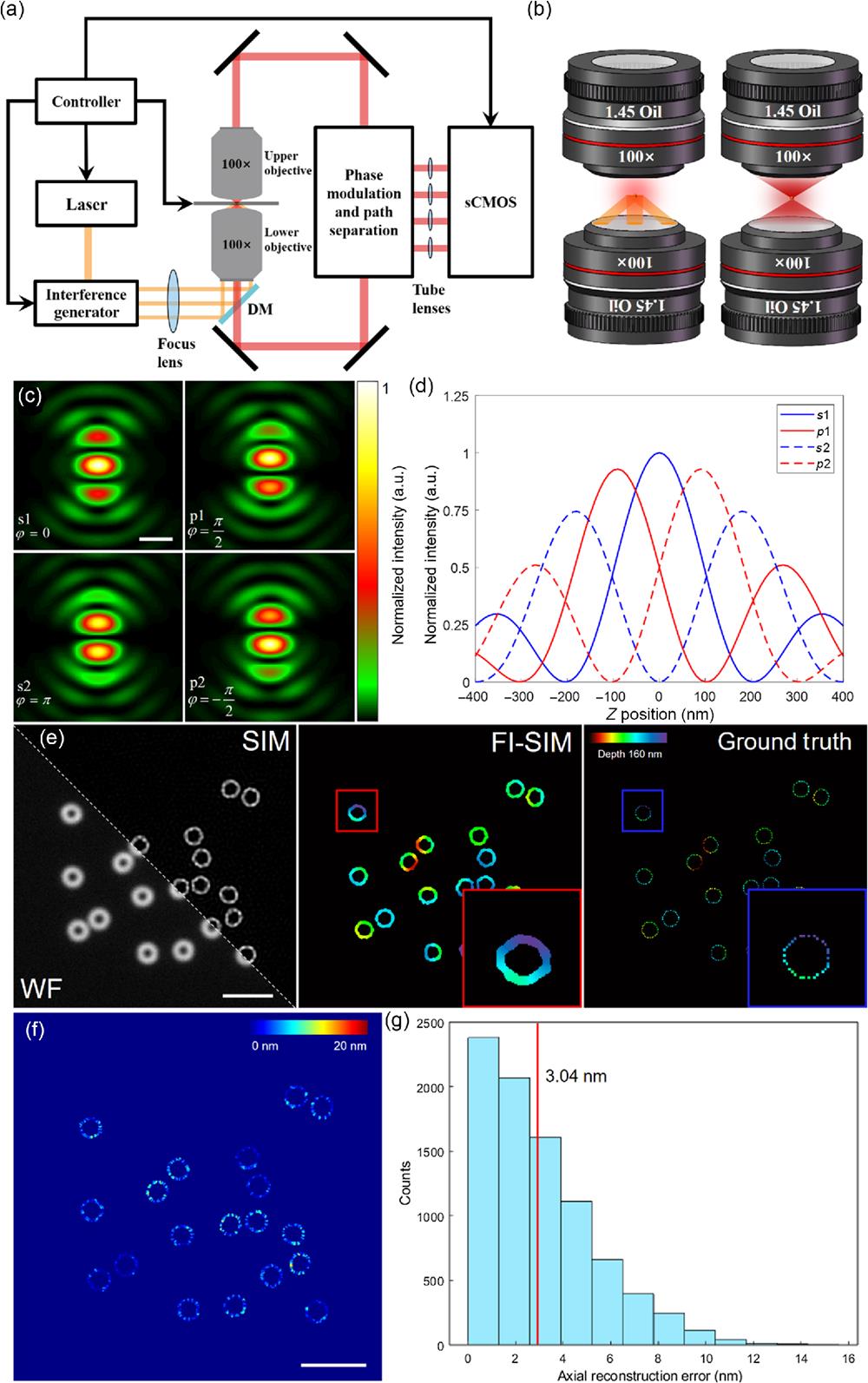
Figure 1.Principle and simulations of FI-SIM. (a) Structure schematic diagram of FI-SIM. Excitation beam was split by the interference generator module, which contains galvo-mirrors and piezo stages to form a three-beam illumination mode (3D-SIM); fluorescence from both upper and lower objectives would interfere and be modulated by phase modulation and path separation modules to form four paths and correspondingly four sub-images, which denoted four different phases of fluorescence interference; the images were collected by sCMOS, and all of the devices were synchronously controlled by computer. (b) Excitation and detection mode of FI-SIM. (Left) For excitation, only the lower objective is used, and the pattern is generated by three-beam illumination, which is the same as 3D-SIM but without axial scanning. (Right) For detection, both objectives collect the fluorescence from the sample, resulting in fluorescence interference. (c) 4Pi PSF of four sub-images with four phases (
In our imaging scheme, a recently established 3D-SIM algorithm named HiFi-SIM34 was used to obtain a single-frame 3D-SIM image from wide-field raw SIM images. (Four sub-images of each acquisition were summed to form 15 raw images of SIM; refer to Fig. S3 in the Supplementary Material.) This achieved lateral super-resolution and reduced the axial detection range to sub-300 nm (for 560 nm excitation wavelength) through the optical sectioning effect of our new 3D-SIM mode to minimize axial reconstruction errors (refer to Fig. S4 in the Supplementary Material). The 3D-SIM super-resolution image was then segmented into a 2D binary mask that can exclude background, noise, and diffraction-limit information and preserve the super-solved target area from the wide-field images of the four channels (refer to Fig. S3 in the Supplementary Material). After being filtered by a binary mask, the four wide-field images were used for phase unwrapping (refer to Notes S2–S4 in the Supplementary Material) and axial reconstruction from different intensity distributions of the four phases (refer to Fig. S3 in the Supplementary Material). Through phase unwrapping for each subregion, the map of the axial distribution of the sample can be obtained in the range.
2.2 Simulations and Calibration
The reconstruction process was conducted and analyzed through simulations of 3D microtubules and ring-shaped structures. The 4Pi-PSF used in the simulations was generated using vectorial diffraction theory.24,35,36 The intensity distribution of each phase varied periodically according to fluorescence interference and phase modulation [Fig. 1(c)]. It is worth mentioning that, unlike ordinary 3D PSF, 4Pi-PSF possesses a hollow structure and sidelobes.37 As the axial position varied, the phase of fluorescence interference changed correspondingly, and the relative ratio of intensities between the four channels also fluctuated. Thus, we could determine the axial position through the relative ratio. However, when the -position exceeded half the wavelength, the relative intensity of the four channels circulated [Fig. 1(d)], resulting in potential axial localization errors (refer to Fig. S4 in the Supplementary Material). To examine our new theory, we simulated ring-shaped structures, which were randomly generated within an axial range of 160 nm (each ring structure had a diameter of 500 nm, and its 3D posture was random) with a three-beam excitation mode and 4Pi-PSFs [Fig. 1(e)]. That is, 15 raw images were generated, and each image contained four sub-images, which denoted four interference phases (, 0, , ), and the simulated sample was distributed within the 160 nm axial range. From the depth-coded image [Fig. 1(e)], we recovered all full ring-shaped structures with high axial resolution. Through 3D SIM recovery and axial reconstruction from four channels, the surface morphology of the structures can be obtained accurately with lateral resolution of SIM and axial resolution. As shown in Figs. 1(f) and 1(g), the average axial reconstruction accuracy was about 3.04 nm, and the positions with axial reconstruction accuracy better than 10 nm account for 98.9% of the total axial reconstruction. This indicates that FI-SIM has an axial resolution better than 30 nm. The reason for applying 3D-SIM rather than 2D-SIM was explained by Fig. S4 in the Supplementary Material. In addition, the theoretical analysis of axial reconstruction was derived and verified by simulations in Figs. S5, S6, and Note S5 in the Supplementary Material.
We also examined axial reconstruction by imaging a high-density 100 nm fluorescent bead sample (FluoSpheres beads, F8801). In the calibration stage, by adjusting the gesture of the BS in the detection path (refer to Fig. S2 in the Supplementary Material), the interference fringe frequency can be reduced in each sub-image until the frequency is minimized, and the phase in each sub-image is nearly uniform (Video 1). By applying the phase calibration algorithm,33 the phase difference between and polarizations (72.8 deg) can be calculated (refer to Fig. S7 in the Supplementary Material). The sample stage was first adjusted to the horizontal position, and then the single-layer bead sample was imaged and reconstructed [Fig. 2(c)]. After axial reconstruction, it can be found that the axial positions of beads in the field of view (FOV) were very close, indicating ideal phase uniformity [refer to Figs. 2(c) and 2(f) and Fig. S8 in the Supplementary Material]. Then, by adjusting the gesture of the sample stage, a 0.24 deg angle was generated between the sample stage and the direction, that is, a depth difference of theoretically 100 nm from the leftmost to the rightmost of the FOV [Figs. 2(a) and 2(b)], which was reflected in the fluorescence interference phase in each sub-image. The three precision piezoelectric displacement devices under the sample stage guarantee the accuracy of the tilt angle [refer to Fig. S2(c) and Note S1 in the Supplementary Material]. With the axial movement of the interference cavity of the 4Pi configuration, the four sub-images showed shifting fringes along the direction (Video 2). After image reconstruction and axial reconstruction, the depth distribution of the beads also changed along the direction [Figs. 2(d) and 2(g)]. According to this distribution in the axial direction, linear functions of depth varying with positions can be fitted. We showed a depth difference of from leftmost to rightmost, which was close to the theoretical value. It can be proved that FI-SIM can achieve axial resolution close to 20 nm with an axial reconstruction accuracy error of no more than 10 nm [Fig. 2(g)] while maintaining the lateral resolution of SIM [the full width at half maxima (FWHM) was 111.3 nm]. In addition, we also generated various depth differences, such as 50 and 150 nm (refer to Fig. S8 in the Supplementary Material), and the corresponding experimental depth differences were 45 and 148.5 nm, which repeatedly verified the axial reconstruction performance. Obviously, for discrete samples (such as fluorescent beads), the axial resolution of FI-SIM is closer to techniques, such as 4Pi-SMS, and significantly better than 4Pi-SIM, as the improvement of axial resolution of the latter relies on OTF frequency shift, and its step size is often greater than 100 nm when performing axial scanning, which has no advantage compared with FI-SIM.
![]()
Figure 2.Calibration by fluorescent beads and schematic diagram of sample stage tilting. (a) Schematic diagram of 0.24 deg tilting between the sample stage and
Through careful calibration and adjustment, our method enabled mapping of the surface morphology of the sample within a lateral resolution equivalent to SIM and even 20 nm-resolution axial distributions of subcellular structures in the range. In addition to calibrating the phase of fluorescence interference, the fluorescent beads can also be used in the process of aberration correction, which can improve the image quality and reliability of axial reconstruction (refer to Note S10 and Fig. S9 in the Supplementary Material).
3 Cell Imaging
To verify the performance of our method in applications, a series of experiments were conducted. Fixed microtubule networks of BSC cells were first tested (Fig. 3). Labeled with the Abberior STAR Orange, a laser () was used to excite the fluorophores under the 3D-SIM illumination mode. To guarantee the quality of the 3D-SIM, the power of the laser should be kept constant, and the power density of the patterns in every direction should be approximately equal. As for fluorescence interference, the images from the upper and lower objective should be merged, and the 4Pi cavity should be adjusted to “interference area,” where the contrast of fluorescence interference reaches the maximum. By collecting 15 images for each channel, up to 60 images can be acquired in 0.75 s (35 ms exposure time for each acquisition). Both 3D-SIM and axial reconstruction can be performed, and, consequently, a 3D morphology image can be obtained.
![]()
Figure 3.Reconstructed image and 3D volume of microtubules and migrasomes. (a) 3D-SIM image without axial scanning. The top-left of (a) is the corresponding wide-field image. (b) 3D volume super-resolution image of microtubules labeled with STAR Orange in BSC cells. (c) Lateral profile of the white line in (b) and the FWHM is 185.6 nm. (d) 3D visualization of the microtubules using Vutara SRX Viewer. (e) Continuous
With image reconstruction, a super-resolved morphology image can be obtained with optical sectioning. Through image segmentation and classification, the spatial mask of the SIM image was used in axial reconstruction. According to the actual phase difference (refer to Fig. S7 in the Supplementary Material) between the and polarizations, the axial positions of each ROI can be obtained and displayed as both depth-coded visualizations and 3D volumes [Figs. 3(b) and 3(d)]. From the depth-coded images and 3D volumes [refer to Figs. 3(b) and 3(d) and Figs. S10(b) and S10(d) in the Supplementary Material], we measured the growth and distribution of bending microtubule networks that changed continuously in the axial direction from the edge to the center (cell nucleus) of the cell. The axial resolution of the reconstructed volumes was , which can be observed in both the reconstructed image stacks and axial sections [refer to Figs. 3(b) and 3(e), and Figs. S10(b) and S10(d) in the Supplementary Material]. We then imaged the migrasomes38 using this setup. In live L929 cells labeled with DID (), we used the same imaging parameters for microtubule networks to obtain the data of the mitochondrial network [Fig. 3(f)]. Similar to microtubules, the branches of migrasomes were not distributed in the same plane, but formed a 3D structure, which indicates the trajectory of cell movement. It can be noted that there existed discrepancies between the axial resolution of fluorescent beads and fixed cells. That is because the fluorescent beads were sparsely distributed in the FOV. Both microtubules and migrasomes, however, were continuous, which results in the performance of each axial reconstruction being affected by other fluorophores within the sub diffraction limit range.
4 Time-Lapse Imaging
To verify the capability of FI-SIM to explore microcosms, we imaged microtubules and mitochondria in live U2OS cells labeled with Tubulin-Tracker Deep Red and Mito-Tracker Deep Red (), respectively, to study the dynamics of their subcellular structures. By staining U2OS cells, our method was applied to image these live cells. The reconstructed 3D volume images clearly illustrated that the mitochondria in the FOV were distributed within a range of 120 nm (while microtubules were distributed within 260 nm) in the axial direction (Fig. 4).
![]()
Figure 4.Reconstructed results of live-cell time-lapse imaging of microtubules and mitochondria. (a), (f) Wide-field image of microtubules and mitochondria in live U2OS cells labeled with Tubulin-Tracker Deep Red and Mito-Tracker Deep Red, respectively. (b), (g) 3D-SIM image of microtubules and mitochondria. (c), (h) Time-lapse wide-field image sequence of the ROIs marked with red outline in (a) and (f) during 2 min with time interval of one minute. (d), (i) Time-lapse 3D-SIM image sequence of the ROIs marked with the red outlined region in (b) and (g). (e), (j) Time-lapse depth-coded 3D volume image sequence of the ROIs marked as red outlined regions in (b) and (g). Scale bar in (a) and (f):
In this study, we acquired a time-lapse image sequence of live cells at 1-min intervals with an exposure time of 35 ms. A few continuous depth-coded images showed the movement, migration, deformation, fusion, and separation of mitochondrial and microtubule networks after 3D-SIM reconstruction and axial reconstruction, as well as the depth change in the axial direction. As shown in the depth-coded images, although there was no obvious activity in the lateral direction for microtubules, the axial movement can be caught and observed with high axial resolution by our FI-SIM [Figs. 4(c)–4(e)]. As for mitochondria, it can be observed that the axial activities can be conducted along the mitochondrial structure [Figs. 4(h)–4(j)], just like the propagation of waves (as shown by the red arrows). With time, the concave position changed along the direction of mitochondrial growth. Similarly, when two segments of mitochondria were fused, the structures originally distributed at different depths first moved to the same depth and then fused with each other, which is consistent with our common sense and other researches39
To verify the performance of fast image acquisition of FI-SIM, a continuous FI-SIM image sequence of migrasomes in live L929 cells was acquired at a temporal resolution of 0.75 s per volume with an exposure time of 35 ms (Fig. 5). For the convenience of displaying the axial movement of the migrasomes in a short period of time, in Fig. 5, we show the FI-SIM images of migrasomes every five frames (that is, 3.75 s). Even within 15 s, it can be clearly observed that due to the migration of L929 cells, significant axial changes of migrasomes can be observed in the FI-SIM image sequence. This also indicates that the migrasomes are not fixed after production by cells but are rapidly changing and participate in cell life activities. The complete continuous FI-SIM images are shown in Video 3.
![]()
Figure 5.Reconstructed results of live-cell fast image acquisition of migrasomes in live L929 cells labeled with DID. (a) 3D-SIM image of migrasomes in live U2OS cells labeled with Tubulin-Tracker Deep Red. (b) Wide-field image of migrasomes. (c), (d), and (e) Time-lapse FI-SIM morphology image sequence of the different ROIs marked with red outline in (a) with fast image acquisition. Scale bar in (a) and (b):
5 Discussion
In summary, we report FI-SIM, a powerful approach to image dynamic subcellular structures and morphologies of both fixed and live cells. This method combines 3D-SIM and axial reconstruction of fluorescence interference, performing fast and accurate 3D imaging without -axis scanning, which other super-resolution configurations cannot provide. As a result, the proposed method can provide precise axial reconstruction and thin optical sectioning of fine structures using fluorescence interference and phase unwrapping, which make it a promising approach to investigate the morphologies and activities of the fine structures of cells.
In previous SMLM technologies, to solve the problem of axial reconstruction error due to a limited period of fluorescence interference, the high-order Gaussian weighted central moment30 and deformable mirror31 were used to extend the axial detection range, which were both challenging and cumbersome. Owing to the 3D-SIM and 4Pi-PSF, the limited detection range, which has been puzzling the axial reconstruction of fluorescence interference for a long time, has been solved perfectly.
On the other hand, compared with 4Pi-SIM, FI-SIM significantly improves axial resolution to the sub-30 nm scale while reducing the complexity of the excitation path, enabling more accurate axial reconstruction with fast data collection. This is something that existing techniques cannot achieve. Moreover, owing to its fast image acquisition process, dynamic live-cell imaging, especially exploring the minor movement of subcellular structures in the axial direction, can be performed using our configuration. In current methods, such as 4Pi-SMS,30 isoSTED,42,43 and other ultra-high axial-resolution methods,44
6 Appendix: Supplementary Information
Video 1. Fluorescence interference of fluorescent beads without sample tilting (AVI, 15.6 MB [URL: https://doi.org/10.1117/1.AP.5.5.056007.s1]).
Video 2. Fluorescence interference of fluorescent beads with 0.24 deg tilting of sample stage (AVI, 3.78 MB [URL: https://doi.org/10.1117/1.AP.5.5.056007.s2]).
Video 3. Imaging migrasomes of live cells (AVI, 2.08 MB [URL: https://doi.org/10.1117/1.AP.5.5.056007.s3]).
Yile Sun is a PhD candidate in the College of Optical Science and Engineering at Zhejiang University. He received his bachelor’s degree in the College of Optical Science and Engineering at Zhejiang University in 2020. His research fields are 4Pi microscopy and structured illumination microscopy.
Hongfei Zhu is a PhD candidate in the Department of Biomedical Engineering at The Chinese University of Hong Kong. He received his bachelor’s degree in the College of Optical Science and Engineering at Zhejiang University in 2021. His research fields are single molecule localization microscopy and structured illumination microscopy.
Cuifang Kuang received his PhD in the School of Science at Beijing Jiaotong University in 2007. From June of 2007 to January of 2008, he was a postdoctoral researcher at Beijing Institute of Technology. From February of 2008 to February of 2010, he was a postdoctoral researcher in the Department of Mechanical Engineering at the University of South Carolina. From September of 2014 to September of 2015, he was a visiting scholar at Massachusetts Institute of Technology. Now, he is a professor at Zhejiang University in the College of Optical Science and Engineering, with research interests in optical super-resolution imaging and photolithography.
Biographies of the other authors are not available.
References
[19] V. Nechyporuk-Zloy. Principles of Light Microscopy: from Basic to Advanced(2022).
[31] F. Huang et al. Ultra-high resolution 3D imaging of whole cells. Cell, 166, 1028-1040(2016).
[37] M. C. Lang et al. 4Pi microscopy with negligible sidelobes. New J. Phys., 10, 043041(2008).
[49] D. M. Greig, B. T. Porteous, A. H. Seheult. Exact maximum a posteriori estimation for binary images. J. R. Stat. Soc.: Ser. B (Methodol.), 51, 271-279(1989).
[50] B. Stephen et al. Distributed Optimization and Statistical Learning via the Alternating Direction Method of Multipliers(2011).

Set citation alerts for the article
Please enter your email address
© Copyright 2018-2021 | Chinese Laser Press. All Rights Reserved 沪ICP备15018463号-20