
Yile Sun, Hongfei Zhu, Lu Yin, Hanmeng Wu, Mingxuan Cai, Weiyun Sun, Yueshu Xu, Xinxun Yang, Jiaxiao Han, Wenjie Liu, Yubing Han, Xiang Hao, Renjie Zhou, Cuifang Kuang, Xu Liu. Fluorescence interference structured illumination microscopy for 3D morphology imaging with high axial resolution[J]. Advanced Photonics, 2023, 5(5): 056007
- Advanced Photonics
- Vol. 5, Issue 5, 056007 (2023)
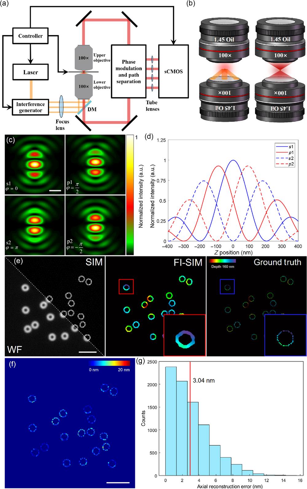
Fig. 1. Principle and simulations of FI-SIM. (a) Structure schematic diagram of FI-SIM. Excitation beam was split by the interference generator module, which contains galvo-mirrors and piezo stages to form a three-beam illumination mode (3D-SIM); fluorescence from both upper and lower objectives would interfere and be modulated by phase modulation and path separation modules to form four paths and correspondingly four sub-images, which denoted four different phases of fluorescence interference; the images were collected by sCMOS, and all of the devices were synchronously controlled by computer. (b) Excitation and detection mode of FI-SIM. (Left) For excitation, only the lower objective is used, and the pattern is generated by three-beam illumination, which is the same as 3D-SIM but without axial scanning. (Right) For detection, both objectives collect the fluorescence from the sample, resulting in fluorescence interference. (c) 4Pi PSF of four sub-images with four phases (
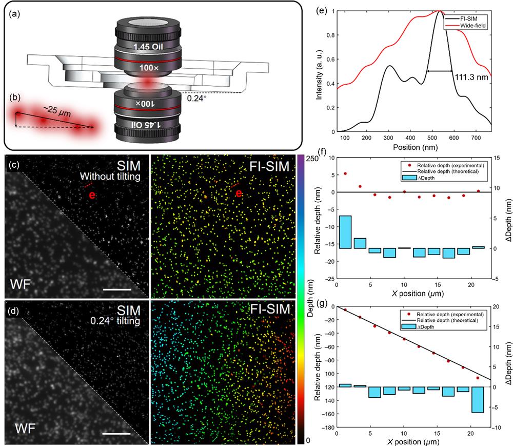
Fig. 2. Calibration by fluorescent beads and schematic diagram of sample stage tilting. (a) Schematic diagram of 0.24 deg tilting between the sample stage and
Fig. 3. Reconstructed image and 3D volume of microtubules and migrasomes. (a) 3D-SIM image without axial scanning. The top-left of (a) is the corresponding wide-field image. (b) 3D volume super-resolution image of microtubules labeled with STAR Orange in BSC cells. (c) Lateral profile of the white line in (b) and the FWHM is 185.6 nm. (d) 3D visualization of the microtubules using Vutara SRX Viewer. (e) Continuous
Fig. 4. Reconstructed results of live-cell time-lapse imaging of microtubules and mitochondria. (a), (f) Wide-field image of microtubules and mitochondria in live U2OS cells labeled with Tubulin-Tracker Deep Red and Mito-Tracker Deep Red, respectively. (b), (g) 3D-SIM image of microtubules and mitochondria. (c), (h) Time-lapse wide-field image sequence of the ROIs marked with red outline in (a) and (f) during 2 min with time interval of one minute. (d), (i) Time-lapse 3D-SIM image sequence of the ROIs marked with the red outlined region in (b) and (g). (e), (j) Time-lapse depth-coded 3D volume image sequence of the ROIs marked as red outlined regions in (b) and (g). Scale bar in (a) and (f):
Fig. 5. Reconstructed results of live-cell fast image acquisition of migrasomes in live L929 cells labeled with DID. (a) 3D-SIM image of migrasomes in live U2OS cells labeled with Tubulin-Tracker Deep Red. (b) Wide-field image of migrasomes. (c), (d), and (e) Time-lapse FI-SIM morphology image sequence of the different ROIs marked with red outline in (a) with fast image acquisition. Scale bar in (a) and (b):

Set citation alerts for the article
Please enter your email address
© Copyright 2018-2021 | Chinese Laser Press. All Rights Reserved 沪ICP备15018463号-20