• Advanced Photonics
  • Vol. 2, Issue 3, 036005 (2020)
Shan Jiang1、2、3, Meiling Guan1, Jiamin Wu4, Guocheng Fang5, Xinzhu Xu1, Dayong Jin2、5, Zhen Liu5, Kebin Shi6, Fan Bai7, Shu Wang8, and Peng Xi1、2、*
Author Affiliations
  • 1Peking University, College of Engineering, Department of Biomedical Engineering, Beijing, China
  • 2Southern University of Science and Technology China, Department of Biomedical Engineering, Shenzhen, Guangdong, China
  • 3Beijing Institute of Collaborative Innovation (BICI), Beijing, China
  • 4Tsinghua University, Department of Automation, Beijing, China
  • 5University of Technology Sydney, Faculty of Science, Institute for Biomedical Materials & Devices (IBMD), Ultimo, Australia
  • 6Peking University, School of Physics, Beijing, China
  • 7Peking University, School of Life Sciences, Biodynamic Optical Imaging Center (BIOPIC), Beijing, China
  • 8Peking University People’s Hospital Breast Center, Beijing, China
  • show less
    DOI: 10.1117/1.AP.2.3.036005 Cite this Article Set citation alerts
    Shan Jiang, Meiling Guan, Jiamin Wu, Guocheng Fang, Xinzhu Xu, Dayong Jin, Zhen Liu, Kebin Shi, Fan Bai, Shu Wang, Peng Xi. Frequency-domain diagonal extension imaging[J]. Advanced Photonics, 2020, 2(3): 036005 Copy Citation Text show less
    An illustration of the FDDE microscopy. (a) Illustration of the sampling interval of an image sensor with a rectangular pixel in the horizontal and diagonal directions. (b) The frequency domain of an image sensor and the OTF of an imaging system in undersampled digital imaging. The green-dash rectangle is the frequency domain of the microscopic image. The yellow-dot circle is the OTF of an imaging system. The green-line rectangle is the frequency domain of undersampled digital imaging. D and H denote the diagonal and horizontal directions, respectively. The spatial domain image of (b) is shown in the upper-right corner. (c) The optical setup of FDDE LFM. (d) Illustration of the frequency stitching algorithm of FDDE.
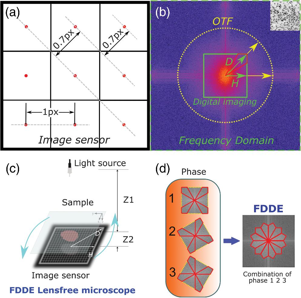
    Fig. 1. An illustration of the FDDE microscopy. (a) Illustration of the sampling interval of an image sensor with a rectangular pixel in the horizontal and diagonal directions. (b) The frequency domain of an image sensor and the OTF of an imaging system in undersampled digital imaging. The green-dash rectangle is the frequency domain of the microscopic image. The yellow-dot circle is the OTF of an imaging system. The green-line rectangle is the frequency domain of undersampled digital imaging. D and H denote the diagonal and horizontal directions, respectively. The spatial domain image of (b) is shown in the upper-right corner. (c) The optical setup of FDDE LFM. (d) Illustration of the frequency stitching algorithm of FDDE.
    LFM imaging with different directions of the image sensor. (a) and (b) The reconstructed hologram images of LFM in the horizontal and diagonal directions, respectively. (c) and (d) The frequency domain of the reconstructed images in (a) and (b), respectively. The dotted rectangle marked in (d) represents the effective frequency boundaries in (c). (e) and (f) The line profiles (element 3 of group 8) marked in (a) and (b), respectively. The red dotted line profile in (f) is the same location in the image that filtered the high frequency out of the yellow rectangle, as illustrated by the inset in (d). The yellow arrows indicate the direction of the sample.
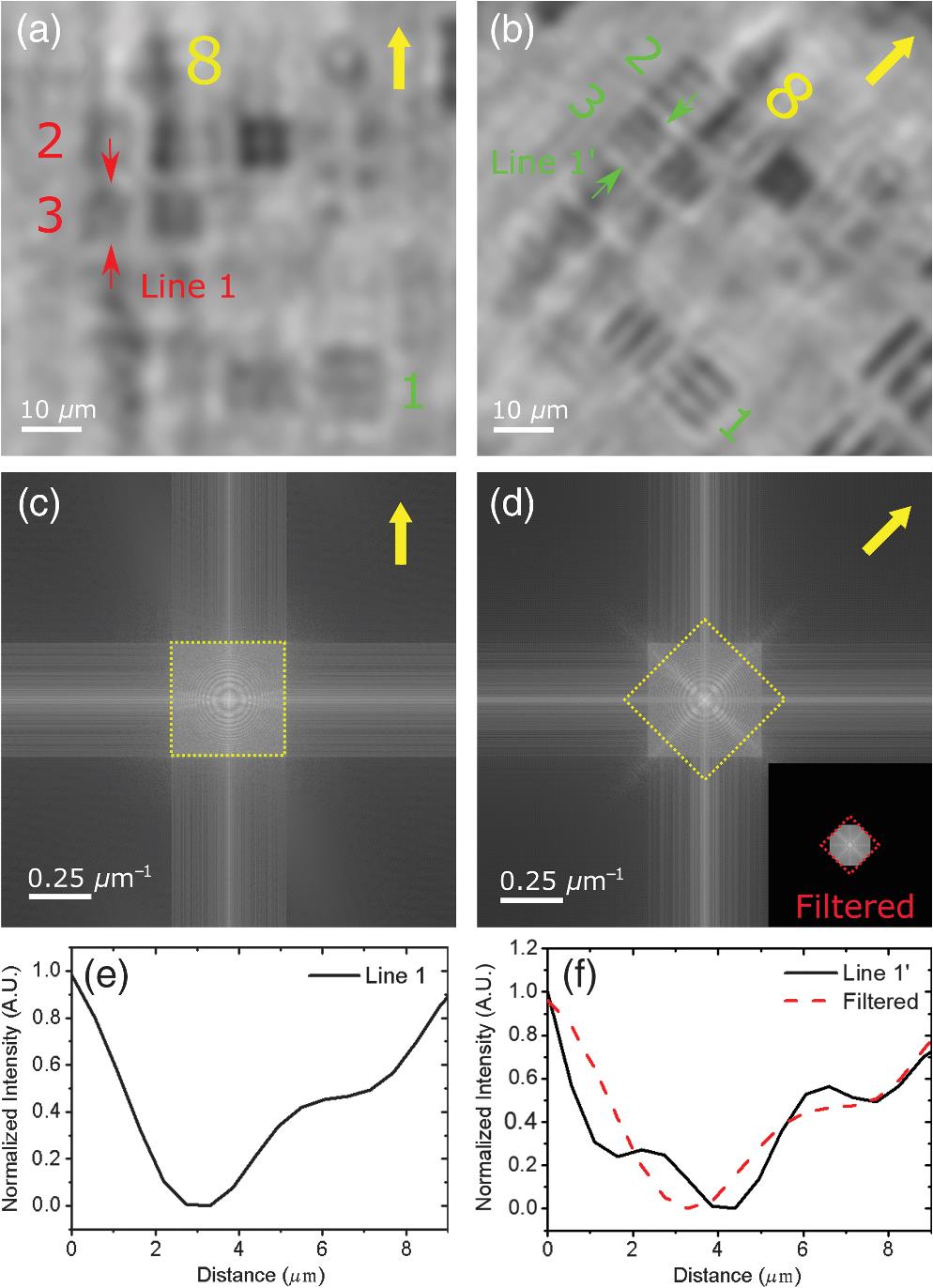
    Fig. 2. LFM imaging with different directions of the image sensor. (a) and (b) The reconstructed hologram images of LFM in the horizontal and diagonal directions, respectively. (c) and (d) The frequency domain of the reconstructed images in (a) and (b), respectively. The dotted rectangle marked in (d) represents the effective frequency boundaries in (c). (e) and (f) The line profiles (element 3 of group 8) marked in (a) and (b), respectively. The red dotted line profile in (f) is the same location in the image that filtered the high frequency out of the yellow rectangle, as illustrated by the inset in (d). The yellow arrows indicate the direction of the sample.
    Demonstration of FDDE imaging with a mouse skin sample. (a) The FDDE LFM image of the mouse skin sample. (b) An enlarged view of the region marked in (a). (c) LFM images. (c1), (c2), and (c3) are the same area as (c4) in the three-phase images with different orientations. The arrows in the upper-right corner correspond to the direction of the sample in the experiment. The three arrows indicate the FDDE image. In addition, (c2) and (c3) and (d2) and (d3) are rotated back to the same direction as in (c1) and (d1), respectively, for a comparison. The line profile in (c4) is marked between the arrows. The inset in (c4) is imaged with a 10× bright-field microscope, presented as the ground truth. (d) The frequency domains of the three-phase images and the FDDE image. The yellow rectangle is the boundary of the lensfree microscope. The red line area in (d1)–(d3) is combined into (d4) based on the principle of FDDE.
    Fig. 3. Demonstration of FDDE imaging with a mouse skin sample. (a) The FDDE LFM image of the mouse skin sample. (b) An enlarged view of the region marked in (a). (c) LFM images. (c1), (c2), and (c3) are the same area as (c4) in the three-phase images with different orientations. The arrows in the upper-right corner correspond to the direction of the sample in the experiment. The three arrows indicate the FDDE image. In addition, (c2) and (c3) and (d2) and (d3) are rotated back to the same direction as in (c1) and (d1), respectively, for a comparison. The line profile in (c4) is marked between the arrows. The inset in (c4) is imaged with a 10× bright-field microscope, presented as the ground truth. (d) The frequency domains of the three-phase images and the FDDE image. The yellow rectangle is the boundary of the lensfree microscope. The red line area in (d1)–(d3) is combined into (d4) based on the principle of FDDE.
    Analysis of FDDE imaging with a blood smear specimen. (a) The FDDE image with the blood smear specimen. (b) An enlarged view of the region marked in (a). (c1)–(c3) The conventional LFM of different angles, and (c4) is the LFM with FDDE. The thick arrows in the upper-right corner correspond to the direction of the sample in the experiment in (c1)–(c3). The three arrows indicate the combined FDDE image in (c4). (d) The bright-field image of the same area, presented as the ground truth. (e) The line profile from (c1)–(c4) marked in (c4).
    Fig. 4. Analysis of FDDE imaging with a blood smear specimen. (a) The FDDE image with the blood smear specimen. (b) An enlarged view of the region marked in (a). (c1)–(c3) The conventional LFM of different angles, and (c4) is the LFM with FDDE. The thick arrows in the upper-right corner correspond to the direction of the sample in the experiment in (c1)–(c3). The three arrows indicate the combined FDDE image in (c4). (d) The bright-field image of the same area, presented as the ground truth. (e) The line profile from (c1)–(c4) marked in (c4).
    Lens-based photography with different orientations of ISO 12233 resolution target. (a) and (b) The interpolated images captured with conventional lens and sCMOS chip. (c) and (d) The line profiles marked in (a) and (b), respectively.
    Fig. 5. Lens-based photography with different orientations of ISO 12233 resolution target. (a) and (b) The interpolated images captured with conventional lens and sCMOS chip. (c) and (d) The line profiles marked in (a) and (b), respectively.
    Shan Jiang, Meiling Guan, Jiamin Wu, Guocheng Fang, Xinzhu Xu, Dayong Jin, Zhen Liu, Kebin Shi, Fan Bai, Shu Wang, Peng Xi. Frequency-domain diagonal extension imaging[J]. Advanced Photonics, 2020, 2(3): 036005
    Download Citation