Diagnostics of the topological charge of optical vortex by a phase-diffractive element

Shiyao Fu; Tonglu Wang; Yan Gao; Chunqing Gao

doi:10.3788/COL201614.080501

Abstract

A phase-diffractive optical element is designed to measure the topological charge of optical vortices. We use the scalar diffraction theory to calculate the far-field diffraction patterns. The simulation results show that almost all of the power of the incident beams is diffracted to the same diffraction order, and this approach is also effective for multi-ring optical vortices. We upload this phase-diffractive optical element on the liquid crystal spatial light modulator to do the experiment. The observed far-field diffraction patterns fit well with the simulation results.

Optical vortices carrying orbital angular momentum (OAM) such as the Laguerre-Gaussian (LG) beams and the Bessel beams are widely used in a lot of fields, including optical tweezers^[1], optical manipulation^[2], optical trapping and guiding of cold atoms^[3,4], generating vector beams^[5], quantum communication^[6], optical communications^[7–10], etc. The eigenvalue of OAM in a single photon is called the topological charge $l$ . Optical vortices with different $l$ values are orthogonal to one another in the Hilbert space, and the value of $l$ is unlimited in theory^[11]. This means optical vortices have the potential to increase the capacity of communication systems^[7,10]. Therefore, measuring the topological charge $l$ is very important.

A number of techniques to detect the topological charge of optical vortices have been reported^[12–16]. Approaches that utilize amplitude diffractive optical elements, including composite fork shaped grating^[17–19] and triangular slit^[20,21], are demonstrated. Methods such as the multipoint interferometer^[22], double-angular-slit interference^[23], Dammann vortex grating^[24–26], Fourier transformation of intensity^[27,28], tilted lens^[29,30], and plasmonic photodiodes^[31] are also reported. Recently, our group designed a new kind of grating with a gradually-changing-period to measure the topological charge^[32]. This method reduces the difficulty of adjusting the optical system, and the diffraction patterns of this grating are easily observed, which meets our demand of the diagnostics of low-order single-ring optical vortices. However, as for multi-ring optical vortices or high-order optical vortices (Ref. [32] just accomplishes the topological charge measurement of a single-ring optical vortex from $- 4$ to $+ 4$ ), this method will not work very well because of the low diffraction efficiency. In addition, the gradually-changing-period grating is an amplitude grating, which means we must use it after production.

On this account, we design a new kind of diffractive optical element based on the gradually-changing-period grating mentioned above. The element we demonstrate can be regarded as a phase grating. On one hand, this optical element can modulate the phase of the incident light beam to realize wavefront division and concentrate most of the energy of the incident optical vortex on the same diffraction order. On the other hand, we can upload the hologram of this diffractive optical element on the liquid crystal spatial light modulator (LC-SLM), which is very easy to operate in practical measurement. In particular, the phase element can realize the measurement of an optical vortex with an arbitrary topological charge in theory.

Sign up for Chinese Optics Letters TOC. Get the latest issue of Chinese Optics Letters delivered right to you！Sign up now

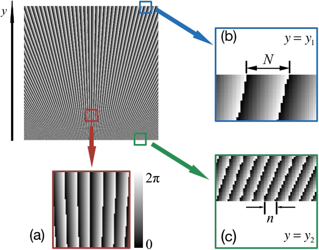
The phase profile of the diffractive optical element can be expressed as $ϕ (x, y) = 2 π \cdot frac (\frac{x}{a + b y}),$ (1)where “frac” means taking the fractional part of a number. Parameters $a$ and $b$ are two basic parameters, which are related to the gradient coefficient of the optical element. The diffractive optical element is shown in Fig. 1(a).

$Phase profile of the diffractive optical element.$

Figure 1.Phase profile of the diffractive optical element.

Now we will discuss how to determine the values of parameters $a$ and $b$ . Assuming that the maximum of the $y$ coordinates in the optical element is $y_{1}$ and the minimum is $y_{2}$ , the grating period on the location of $y = y_{1}$ is $N$ , on the location of $y = y_{2}$ is $n$ , and $N > n$ , as illustrated in Figs. 1(b) and 1(c). The grating constant is a linear function of $y$ in this optical element. So we can get a first-order linear equation set about parameters $a$ and $b$ , ${\begin{matrix} N = a + b y_{1}, \\ n = a + b y_{2}, \end{matrix}$ (2)and by solving Eq. (2) can we get the value of parameters $a$ and $b$ .

The scalar diffraction theory and the fast Fourier transform (FFT) algorithm are used to analyze the far-field diffraction patterns when optical vortices are incident in this diffractive optical element. The detection system we design satisfies the paraxial approximation. Therefore, we can use Fresnel diffraction to simplify the diffraction integral formula. However, it may cause some problems because Fresnel diffraction is not applicable in the calculation of the far-field diffraction, but it is good for the finite propagation distance, and what we want is the far-field diffraction patterns. So, we add a convex lens to the optical element to compensate for when we calculate the diffraction result. The Fresnel diffraction integral can be written as $U (x, y) = \frac{\exp (j k d)}{j λ d} \iint_{\infty} U_{0} (x_{0}, y_{0}) \cdot \exp {\frac{j k}{2 d} [{(x - x_{0})}^{2} + {(y - y_{0})}^{2}]} d x_{0} d y_{0},$ (3)where $U_{0} (x_{0}, y_{0})$ is the complex amplitude of the incident beam, $U (x, y)$ is the optical field behind the optical element in the observation plane, $d$ is the distance between the optical element and the observation plane, $λ$ is the wavelength, and $k$ is the wave number. Equation (3) can be simplified again with the help of the Fourier transform^[33], which can be written as $U (x, y) = F^{- 1} {F [U_{0} (x_{0}, y_{0})] \cdot \exp [j k d (1 - \frac{x^{2} + y^{2}}{2 d^{2}})]},$ (4)where $F$ and $F^{- 1}$ are the Fourier transformation and the Fourier inversion, respectively. Equation (4) allows us to use the FFT to analyze the diffraction, and it will make the calculation easier. Under the condition of paraxial approximation, the phase profile of the spherical lens can be written as $φ (x, y) = k \cdot \frac{x^{2} + y^{2}}{2 f},$ (5)where $f$ is the focal length of the lens, which is equal to the $d$ in Eq. (4), so as to realize the calculation of the far-field diffraction. Here we use LG mode as the incident optical vortex. The LG mode is the single-ring optical vortex when the radial index $p = 0$ . When $p \neq 0$ , it is the multi-ring optical vortex. Assuming that the complex amplitude of the incident optical vortex is $G$ , then $U_{0}$ can be expressed as $U_{0} = G \exp (i ϕ) \cdot \exp (i φ) .$ (6)

The far-field diffraction patterns can be obtained when we plug Eqs. (1), (5), and (6) into Eq. (4). The software MATLAB is used here to help us to realize the calculation of the above equations. In our simulation, the basic parameters of the optical element are set as $N = 0.4 mm$ and $n = 0.2 mm$ . The waist radius of the fundamental Gaussian mode is 1.5 mm. Figure 2 shows the incident optical vortices and the far-field diffraction patterns when the optical vortices propagate through the optical element we design. The diffraction patterns are similar to the Hermite-Gaussian (HG) modes. The spot number of them is related to the absolute value of the incident beams’ topological charge, which can be expressed as $(| l | + p + 1) \cdot (p + 1)$ . Hence, $| l |$ can be written as $| l | = [W / (p + 1) - (p + 1)],$ (7)where $W$ is the number of spots. The orientation of the spots (horizontal or vertical) is related to the sign of the topological charge. The phenomena above mean that this optical element can realize the measurement of the topological charge. First, we can verify the radial index $p$ by detecting the incident optical vortex (the number of rings minus one is $p$ ). Second, the orientation of the spots tells us the sign of the topological charge: vertical means positive, and horizontal means negative. Third, the number of spots tells us the absolute value of the topological charge (Eq. (7)). We list a couple of examples of the measurement procedure of this diffracted optical element, as shown in Fig. 3. Figure 2 also shows that almost all of the power of the incident beams is diffracted to the same diffraction order. This is different from the gradually-changing-period grating of which just about 10% of the incident power is diffracted to the first diffraction order that we need^[32].

$Normalized intensity distribution of the incident optical vortices and the simulated far-field diffraction patterns. (a), (b), and (c) are the incident single-ring (radial index p=0) optical vortices with topological charge l=1, l=−1, and l=2, respectively. (d) and (e) are the incident multi-ring incident optical vortices with topological charge l=1 and l=−1. (f), (g), (h), (i), and (j) are the simulation results of the normalized intensity distribution of the far-field diffraction when the optical vortices shown in (a), (b), (c), (d), and (e) propagate through the diffractive optical element, respectively. (k) and (l) are the 3D images of the normalized intensity distributions of (c) and (h).$

Figure 2.Normalized intensity distribution of the incident optical vortices and the simulated far-field diffraction patterns. (a), (b), and (c) are the incident single-ring (radial index $p = 0$ ) optical vortices with topological charge $l = 1$ , $l = - 1$ , and $l = 2$ , respectively. (d) and (e) are the incident multi-ring incident optical vortices with topological charge $l = 1$ and $l = - 1$ . (f), (g), (h), (i), and (j) are the simulation results of the normalized intensity distribution of the far-field diffraction when the optical vortices shown in (a), (b), (c), (d), and (e) propagate through the diffractive optical element, respectively. (k) and (l) are the 3D images of the normalized intensity distributions of (c) and (h).

Figure 3.Two examples of the detecting procedure of our method. (a) The case of a single-ring optical vortex with $l = + 4$ . (b) The case of a multi-ring optical vortex with $l = - 2$ .

We build an experimental setup to measure the topological charge practically, as sketched in Fig. 4. The diameter of the collimator is 3 mm, and the LD’s output power is about 20 mW. Two LC-SLMs by Holoeye are used here to create the desired phase profiles. Their active area is $15.36 mm \times 8.64 mm$ , the resolution nominal is $1920 \times 1080 pixels$ and the pixel pitch is 8.0 μm. The LC-SLM we use can be programmed in any desired phase profile for horizontal linearly polarized monochromatic light. So adding a polarized beam splitter (PBS) before SLM1 is necessary. Of course, the PBS here can be replaced by a horizontal polarizer. In this experiment, SLM1 is used to generate an optical vortex. The computer-generated holograms of the spiral phase plate are calculated, and then uploaded to SLM1. When the Gaussian beam whose wavelength is 1550 nm that is emitted by an LD is incident at SLM1, the emergent light beams are LG beams. Figure 5 displays the holograms of different kinds of spiral phase plates and their simulation results of far-field distributions when the Gaussian beam propagates through them. The phase-diffractive optical element is uploaded on SLM2 to realize the measurement of the topological charge. An infrared CCD camera whose spectrum range is 900–1700 nm is placed at the focal plane of the convex lens, and is used to observe the far-field diffraction pattern. We upload nothing on SLM2 at first in order to detect the incident optical vortex. After that, the hologram of the phase grating we designed is uploaded, and the far-field diffraction patterns are attained by an infrared CCD camera.

Figure 4.Experimental setup to diagnose the topological charge of the optical vortex. LD, laser diode; SMF, single mode fiber; Col., collimator; L, convex lens.

$Holograms of the spiral phase plate and the simulation results of the generated LG modes. From (a) to (e) are the spiral phase plates to generate the LG0–1 mode, LG05 mode, LG1–1 mode, LG13 mode, and LG21 mode, separately. (f), (g), (h), (i), and (j) are the simulation results of the far-field diffraction patterns when the Gaussian beams propagate through the holograms above.$

Figure 5.Holograms of the spiral phase plate and the simulation results of the generated LG modes. From (a) to (e) are the spiral phase plates to generate the ${LG}_{0 - 1}$ mode, ${LG}_{05}$ mode, ${LG}_{1 - 1}$ mode, ${LG}_{13}$ mode, and ${LG}_{21}$ mode, separately. (f), (g), (h), (i), and (j) are the simulation results of the far-field diffraction patterns when the Gaussian beams propagate through the holograms above.

Figure 6 displays the far-field diffraction patterns when the single-ring optical vortices are incident. In each submap, the first row is the incident optical vortices, the second row is the simulation results of the far-field diffraction patterns when the optical vortices in the first row are incident, and the third row is the patterns observed by the CCD camera in the experiment.

Figure 6.Experimental results of the incident single-ring optical vortices. (a) The case of the optical vortices with a positive topological charge. (b) The case of the optical vortices with a negative topological charge. In each submap, from top to bottom are the incident optical vortices, simulation results, and experimental results, respectively.

The condition of the multi-ring optical vortices is shown in Fig. 7. In this case, the radial index $p \neq 0$ . The incident multi-ring optical vortices are the ${LG}_{11}$ mode, ${LG}_{1 - 1}$ mode, ${LG}_{13}$ mode, ${LG}_{21}$ mode, and ${LG}_{2 - 1}$ mode from top to bottom, respectively.

Figure 7.Experimental results of the incident multi-ring optical vortices. From left to right are the ${LG}_{11}$ mode, ${LG}_{1 - 1}$ mode, ${LG}_{13}$ mode, ${LG}_{21}$ mode, and ${LG}_{2 - 1}$ mode, separately. From top to bottom are the incident multi-ring optical vortices, simulation results, and experimental results, respectively.

We can easily find that the experimental results shown in Figs. 6 and 7 fit well with the simulation results, which strongly suggest that the diffractive optical element we demonstrated can be used to diagnose the topological charge. The incident optical vortices are diffracted by the phase-diffractive optical element, and the far-field diffraction patterns have the structure that is similar with the HG modes. The topological charge of the arbitrary single-ring or multi-ring optical vortices can be measured very effectively. What we should do is to judge the orientation and the number of the spots in the far-field diffraction patterns.

Compared with the other diagnostic methods of optical vortices, the great improvement of this phase-diffraction optical element is the detection of the multi-ring optical vortices (the radial index $p \neq 0$ ), and the fabrication of this element is unnecessary. We just need to upload the hologram of the optical element on the LC-SLM, which makes it more convenient in practice. It is available for realizing the detection of optical vortices in a weak intensity because almost all of the energy of the incident light is diffracted to the same diffraction order. However, this approach also has some limits. It can accomplish the diagnostics of the arbitrary order of the single mode optical vortices in theory, but it is not available for the coaxial multiplexing optical vortices.

In conclusion, it is the first time to the best of our knowledge for the demonstration of a method using a phase optical element with a gradually-changing-period to realize the diagnostics of the topological charge of optical vortices. The method is very efficient and convenient, which can be used in the fields of optical communications, optical tweezers, and so on.

References

[1] A. Ashkin, J. M. Dziedzic, J. E. Bjorkholm, S. Chu. Opt. Lett., 11, 288(1986).

[2] M. Padgett, R. Bowman. Nat. Photon., 5, 343(2011).

[3] X. Xu, K. Kim, W. Jhe, N. Kwon. Phys. Rev. A, 63, 063401(2001).

[4] M. Gao, C. Gao, Z. Lin. Chin. Opt. Lett., 5, 89(2007).

[5] S. Fu, C. Gao, Y. Shi, K. Dai, L. Zhong, S. Zhang. Opt. Lett., 40, 1775(2015).

[6] A. Nicolas, L. Veissier, L. Giner, E. Giacobino, D. Maxein, J. Laurat. Nat. Photon., 8, 234(2014).

[7] J. Wang, J. Y. Yang, I. M. Fazal, N. Ahmed, Y. Yan, H. Huang, Y. Ren, Y. Yue, S. Dolinar, M. Tur, A. E. Willner. Nat. Photon., 6, 488(2012).

[8] M. Zhang, P. Jia, Y. Li, T. Lei, Z. Li, X. Yuan. Chin. Opt. Lett., 13, 100502(2015).

[9] M. J. Willner, H. Huang, N. Ahmed, G. Xie, Y. Ren, Y. Yan, M. P. J. Lavery, M. J. Padgett, M. Tur, A. E. Willner. Opt. Lett., 38, 5240(2013).

[10] H. Huang, G. Xie, Y. Yan, N. Ahmed, Y. Ren, Y. Yue, D. Rogawski, M. J. Willner, B. I. Erkmen, K. M. Birnbaum, S. J. Dolinar, M. P. J. Lavery, M. J. Padgett, M. Tur, A. E. Willner. Opt. Lett., 39, 197(2014).

[11] L. Allen, M. W. Beijersbergen, R. J. C. Spreeuw, J. P. Woerdman. Phys. Rev. A, 45, 8185(1992).