• Advanced Photonics
  • Vol. 2, Issue 5, 056003 (2020)
Vitali Kozlov1、*, Sergei Kosulnikov1, Dmytro Vovchuk1、2, and Pavel Ginzburg1
Author Affiliations
  • 1Tel Aviv University, School of Electrical Engineering, Tel Aviv, Israel
  • 2Yuriy Fedkovych Chernivtsi National University, Department of Radio Engineering and Information Security, Chernivtsi, Ukraine
  • show less
    DOI: 10.1117/1.AP.2.5.056003 Cite this Article Set citation alerts
    Vitali Kozlov, Sergei Kosulnikov, Dmytro Vovchuk, Pavel Ginzburg. Memory effects in scattering from accelerating bodies[J]. Advanced Photonics, 2020, 2(5): 056003 Copy Citation Text show less
    Illustration of memory effects on wave–matter interaction in accelerating reference frames. A specific example is an incident pulse scattered from a rotating dipole with memory. Slow relaxation rates permit the excitation of the dipole at one moment to decay when the scatterer had changed its position significantly. The scattering process may be thought of as an LTV process, where non-Markovian behavior manifests in nontrivial signatures at the scattered far field.
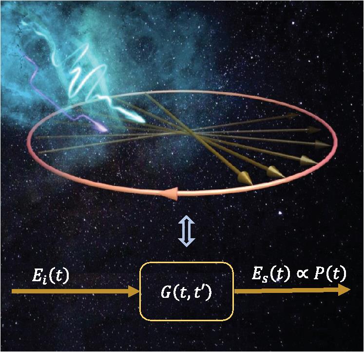
    Fig. 1. Illustration of memory effects on wave–matter interaction in accelerating reference frames. A specific example is an incident pulse scattered from a rotating dipole with memory. Slow relaxation rates permit the excitation of the dipole at one moment to decay when the scatterer had changed its position significantly. The scattering process may be thought of as an LTV process, where non-Markovian behavior manifests in nontrivial signatures at the scattered far field.
    Comparison between the exact and quasistationary (adiabatic, timescale separation) solutions. (a) The spectrum of the induced dipole moment contains two frequencies. The memoryless solution [Eq. (6)] has equal amplitudes and phases while the scattering from a dipole with memory [Eq. (9)] has an asymmetric spectrum. Inset: a dipole, rotating with angular frequency θ˙. (b), (c) The behavior of the amplitude and phase of the spectral peaks, for high and low Q factors, as a function of dimensionless rotation frequency Ω=θ˙γ.
    Fig. 2. Comparison between the exact and quasistationary (adiabatic, timescale separation) solutions. (a) The spectrum of the induced dipole moment contains two frequencies. The memoryless solution [Eq. (6)] has equal amplitudes and phases while the scattering from a dipole with memory [Eq. (9)] has an asymmetric spectrum. Inset: a dipole, rotating with angular frequency θ˙. (b), (c) The behavior of the amplitude and phase of the spectral peaks, for high and low Q factors, as a function of dimensionless rotation frequency Ω=θ˙γ.
    Experimental setup for probing scattering from rotating objects. (a) The schematic representation of the setup. A carrier frequency ω is split between a transmitting and a receiving arm. The transmitting arm is mixed with a Gaussian (G) pulsed signal of controllable pulse length to generate the envelope. The receiving arm is split into two quadratures in order to down-convert the scattered signal. (b) A photo of the experimental setup inside the anechoic chamber. Inset: enlarged photograph of the mechanism to control the wire’s rotation (electric dipole analogue; rotation direction is marked with red arrow) at a constant frequency of 3.4 Hz.
    Fig. 3. Experimental setup for probing scattering from rotating objects. (a) The schematic representation of the setup. A carrier frequency ω is split between a transmitting and a receiving arm. The transmitting arm is mixed with a Gaussian (G) pulsed signal of controllable pulse length to generate the envelope. The receiving arm is split into two quadratures in order to down-convert the scattered signal. (b) A photo of the experimental setup inside the anechoic chamber. Inset: enlarged photograph of the mechanism to control the wire’s rotation (electric dipole analogue; rotation direction is marked with red arrow) at a constant frequency of 3.4 Hz.
    Far-field scattering of Gaussian pulses from a rotating wire, comparing short memory (adiabatic, quasistationary) simulation with experiment (the setup appears in Fig. 3). Blue lines: two different Gaussian pulse lengths, 0.3536 and 0.1414 s measured experimentally. Red lines: numerical analysis using the short-memory method. Black dashed-dotted line: the envelope of the incident pulse [panels (a) and (b)] and its spectrum [panels (b) and (d)]. Columns: scattered signals in time and frequency domains, respectively.
    Fig. 4. Far-field scattering of Gaussian pulses from a rotating wire, comparing short memory (adiabatic, quasistationary) simulation with experiment (the setup appears in Fig. 3). Blue lines: two different Gaussian pulse lengths, 0.3536 and 0.1414 s measured experimentally. Red lines: numerical analysis using the short-memory method. Black dashed-dotted line: the envelope of the incident pulse [panels (a) and (b)] and its spectrum [panels (b) and (d)]. Columns: scattered signals in time and frequency domains, respectively.
    Comparison of the scattered baseband spectra obtained in simulation and experiment as a function of frequency and pulse length. As the pulse length increases (in comparison with rotation speed), the micro-Doppler peaks form at discrete frequencies. For short pulses, the peaks are broader in frequency, creating a featureless spectral continuum. The initial angle for both experiment and simulation is taken as θ0=0 deg⁡.
    Fig. 5. Comparison of the scattered baseband spectra obtained in simulation and experiment as a function of frequency and pulse length. As the pulse length increases (in comparison with rotation speed), the micro-Doppler peaks form at discrete frequencies. For short pulses, the peaks are broader in frequency, creating a featureless spectral continuum. The initial angle for both experiment and simulation is taken as θ0=0deg.
    Colormap, demonstrating scattered signals spectra at the baseband. Vertical axis—initial angle between the wire and the polarization of the incident field, horizontal axis—frequency. Different pulse widths are indicated in insets. (a), (c), (e), and (g) Numerical data. (b), (d), (f), and (h) Experimental data.
    Fig. 6. Colormap, demonstrating scattered signals spectra at the baseband. Vertical axis—initial angle between the wire and the polarization of the incident field, horizontal axis—frequency. Different pulse widths are indicated in insets. (a), (c), (e), and (g) Numerical data. (b), (d), (f), and (h) Experimental data.
    Vitali Kozlov, Sergei Kosulnikov, Dmytro Vovchuk, Pavel Ginzburg. Memory effects in scattering from accelerating bodies[J]. Advanced Photonics, 2020, 2(5): 056003
    Download Citation