
Guoliang Yang, Jiaren Gong, Hao Xi, Dingling Yu. Hyperspectral Image Abnormal Target Detection Based on End-Member Extraction and Low-Rank and Sparse Matrix Decomposition[J]. Laser & Optoelectronics Progress, 2021, 58(22): 2228003
- Laser & Optoelectronics Progress
- Vol. 58, Issue 22, 2228003 (2021)
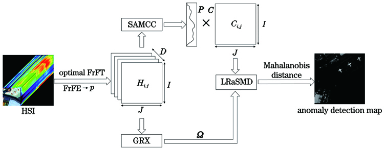
Fig. 1. Framework of our algorithm
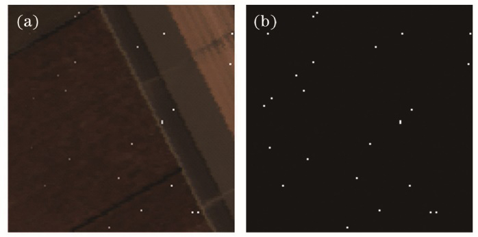
Fig. 2. Salinas synthetic dataset. (a) False-color image; (b) ground-truth map
Fig. 3. SpecTIR dataset. (a) False-color image; (b) ground-truth map
Fig. 4. HYDICE urban dataset. (a) False-color image; (b) ground-truth map
Fig. 5. San Diego dataset. (a) False-color image; (b) ground-truth map
Fig. 6. Output results of different algorithms. (a) Salinas; (b) SpecTIR; (c) HYDICE; (d) San Diego; (e) ABU-A4; (f) ABU-B3; (g) ABU-U1
Fig. 7. ROC curves of different algorithms on Salinas synthetic dataset. (a) ROC curve; (b) logarithmic ROC curve
Fig. 8. ROC curves of different algorithms on SpecTIR dataset. (a) ROC curve; (b) logarithmic ROC curve
Fig. 9. ROC curves of different algorithms on HYDICE urban dataset. (a) ROC curve; (b) logarithmic ROC curve
Fig. 10. ROC curves of different algorithms on San Diego dataset. (a) ROC curve; (b) logarithmic ROC curve
Fig. 11. ROC curves of different algorithms on ABU-A4 dataset. (a) ROC curve; (b) logarithmic ROC curve
Fig. 12. ROC curves of different algorithms on ABU-B3 dataset. (a) ROC curve; (b) logarithmic ROC curve
Fig. 13. ROC curves of different algorithms on ABU-U1 dataset. (a) ROC curve; (b) logarithmic ROC curve
|
Table 1. Parameters of our algorithm on different datasets
|
Table 2. AUC values of different algorithms
|
Table 3. Detection time of different algorithm unit: s

Set citation alerts for the article
Please enter your email address
© Copyright 2018-2021 | Chinese Laser Press. All Rights Reserved 沪ICP备15018463号-20