
Qinghua Gu, Fawen Wei, Mengli Guo, Song Jiang, Shunling Ruan. Segmentation Method of Broken Ore Image Based on Improved HED Network Model[J]. Laser & Optoelectronics Progress, 2022, 59(2): 0210020
- Laser & Optoelectronics Progress
- Vol. 59, Issue 2, 0210020 (2022)
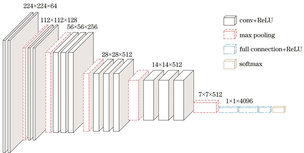
Fig. 1. Structure of VGG network
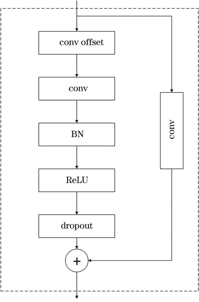
Fig. 2. Structure of deformable convolution module
Fig. 3. Schematic of convolution sampling points. (a) Standard convolution; (b) deformable convolution
Fig. 4. Expansion results of convolution kernel of 3×3 size under different cavity rates. (a) l=1; (b) l=2; (c) l=3
Fig. 5. Framework structure of proposed network
Fig. 6. Images before and after bilateral filtering. (a) Original image of ore; (b) image filtered by 3×3 filtering window
Fig. 7. Relationship among loss, accuracy, and iterations of improved HED network model. (a) Loss; (b) accuracy
Fig. 8. Segmentation results of different network models. (a) Original images; (b) Canny operator; (c) original HED network; (d) improved HED network
|
Table 1. Training parameters of model
| |||||||||||||||||||||||||||||||||||||||||||||||||||||||||||||||||||||||||||||||||||||||||||||||||||||||||||||||||||||||||||||||||
Table 2. Performance indicators of different networks
|
Table 3. Time comparison results of different networks
|
Table 4. Ablation experiment results of different network models

Set citation alerts for the article
Please enter your email address
© Copyright 2018-2021 | Chinese Laser Press. All Rights Reserved 沪ICP备15018463号-20