As a basic parameter of the ocean state equation, the salinity, temperature, and depth of seawater are important parameters for studying the physical ocean^[1–3]. Accurate measurement of these parameters is essential for marine development and utilization^[4]. Traditional salinity, temperature, and depth measurement devices are based on conductivity-temperature-depth measurement systems (CTDs) depending on typical electronic devices^[1]. Although the traditional CTD has the characteristics of high measurement accuracy and wide response range, it is usually expensive, bulky, and susceptible to electromagnetic interference, and cannot be used near the surface of seawater^[1–5]. Therefore, in recent years, optical fiber sensors with small size, low cost, convenient multiplexing, and anti-electromagnetic interference have attracted attention^[6], such as Bragg grating fibers, Fabry–Perot fiber interferometers, dual-core fibers, photonic crystals, plastic fibers, and microfibers (MFs)^[6–13].

The trend of ocean parameter measurement is high efficiency and low cost, but most of these sensors are complex and low in sensitivity, which limits their popularization and application^[3]. In recent years, based on a large proportion of evanescent field transmission characteristics, novel MF sensing technology, such as the MF and MF coupler (MC), which measures air humidity^[14], temperature^[15], and magnetic field^[16–18], has been widely used in various physical parameter sensing because of its small size, high sensitivity, simple fabrication, low cost, and fast response^[19]. More notable is that the realization of high sensitivity sensing of seawater salinity, temperature, and depth based on an MC^[6] indicates the application prospect of MCs in ocean parameter measurement.

However, an MC is a four-port, straight-through photonic device (excessive ports exist for sensing applications). Therefore, the special structure and methods are needed to encapsulate the free ports, which causes inconvenience to the MC-based marine environment parametric sensor design and multiplexing integration, and difficulties to its practical research.

The two output ports of the MC are connected to form a fiber loop (FL), thereby forming an MC combined fiber loop (MCFL) reflective photonic device that can effectively solve the above difficulties. This structure has been used to measure magnetic field strength^[20,21], rotation angle^[22], and refractive index (RI)^[23], but no report has been found for seawater salinity, temperature, and depth measurement.

In this Letter, MCFL samples are prepared. Based on the preliminary analysis of the principle of salinity, temperature, and depth sensing, the three single-parameter experiments are carried out under laboratory conditions. The experimental results show that high-sensitivity salinity, temperature, and depth sensing can be realized based on MCFL. In addition, based on past research experience, the three-parameter synchronous measurement and demodulation may be realized through the cross-sensitivity matrix, and the MCFL-based CTD can be fabricated. This achievement has opened up a good research idea for the development of all-fiber CTD sensors and laid a good research foundation for the practical development of MC-based CTD sensors.

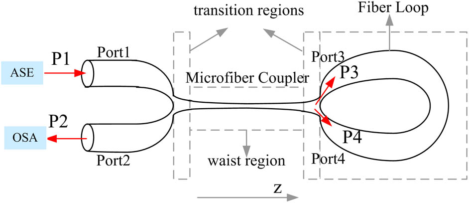
The process of making MCFL is as follows. Bend a single-mode fiber and fold it in half to form an FL^[23]. Strip two fiber claddings at the FL port by about 6 cm, wash with alcohol, and cross the two fibers. Two turns are made to make close contact, the entangled region is laterally melted and tapered to form an MC^[6], and finally the MCFL shown in Fig. 1 is fabricated.

The MC consists of a tapered transition region and a uniform waist region. The coupling process is divided into two parts: transition regions coupling and a uniform waist region coupling. The length of the FL has an influence on the filtering characteristics of the MCFL^[20]. However, the FL used in this Letter is made of conventional single-mode fiber, and the birefringence effect is relatively limited^[24]. When the FL length composed of such fibers is small, its response to the environmental change is much smaller than that of the MC. Therefore, the sensing response of the MC is mainly considered. Since the light passes through the sensing area twice, the resonant peaks of the MCFL are twice that of the MC^[23], making the sensing unit more compact.

Since the coupling region is slowly changing, the coupling characteristics of the MC can be analyzed by the local coupling mode theory^[24,25]; therefore, the output optical power at the Port2 of the MCFL is^[23,24]P2=P0{1−12sin2[2∫0lc(λ,n2,z)dz]}=P0(1−12sin2ϕ),(1)where P0 represents the input light intensity of Port1, l represents the length of the MC, and c(λ,n2,z) represents the coupling coefficient at position z. Under strong coupling conditions, the two tapered MFs are in close contact fusion, and the coupling coefficient can be expressed as^{[6,23,24,26,27]}c(λ,n2,z)=3πλ32n2r21(1+1/V)2,(2)where V=[(2πr)/λ](n22−n32)1/2 denotes the normalized frequency, r is the radius of the waist region MC, λ is the incident wavelength, and n2 and n3 represent the RI of the cladding and the external environment, respectively.

λ is controlled by the amplified spontaneous emission (ASE) source. The parameters n2, n3, l, and r are affected by the surrounding environment. Changes in these parameters will cause the resonant wavelength of the output light to move, and the salinity, temperature, and depth of seawater can be determined by detecting the movement of the characteristic wavelengths^[3,6]. For the characteristic wavelengths at which the output optical power is a maximum value or a minimum value, dP2=0 or dϕ=0, so there is dλ=−∂λ∂ϕ·(∂ϕ∂n3·dn3+∂ϕ∂n2·dn2+∂ϕ∂l·dl+∂ϕ∂r·dr).(3)

Known by Eqs. (1) and (2): ∂ϕ/∂n3<0, ∂ϕ/∂λ>0^[23], ∂ϕ/∂l>0, ∂ϕ/∂r<0. The value of ∂ϕ/∂n2 needs to be analyzed in the experiments of this Letter, n3∈(1.33,1.37), n2=1.486, λ>1520nm, r<3.9μm, therefore ∂ϕ∂n2∝λ(n22+n32)−2πr(n22−n32)32>0.(4)

Unlike traditional electrical CTD, which obtains salinity by measuring conductivity, the MCFL obtains salinity by measuring the ambient RI n3. However, in order to follow the customary term CTD, this Letter still uses “conductivity” to indicate seawater salinity. The increase of seawater salinity (conductivity) will cause the ambient RI n3 to become larger, dn3/dS>0, which has no effect on the cladding RI n2, the coupling length l, and the MC waist radius r. Therefore, its sensitivity response can be expressed as SS=dλdS=−∂λ∂ϕ·∂ϕ∂n3·dn3dS.(5)

Therefore, SS>0, that is, the characteristic wavelength is redshifted with the increase of salinity.

It can be seen from Eq. (3) that the seawater temperature causes the characteristic wavelength to shift by causing a change in the cladding RI n2, the ambient RI n3, the coupling length l, and the MC waist radius r. The response sensitivity formula is ST=dλdT=−∂λ∂ϕ·(∂ϕ∂n3·dn3dT+∂ϕ∂n2·dn2dT+∂ϕ∂l·dldT+∂ϕ∂r·drdT).(6)

Due to the thermo-optic effect, the increase in temperature causes the RI to decrease^[6], and the MC coupling length l and the waist radius r also increase with temperature, so dn3/dT<0, dn2/dT<0, dl/dT>0, and dr/dT>0. Therefore, the ambient RI n3 and the MC coupling length l will cause the characteristic wavelength to blueshift with temperature and the cladding RI n2, and the MC waist radius r will redshift with increasing temperature. However, due to the presence of a large proportion of evanescent fields, the change in the ambient RI n3 plays a dominant role in temperature sensitivity after the sensor is optimized, and an increase in temperature will result in a blueshift in the characteristic spectrum.

The seawater pressure causes the characteristic wavelength to shift by causing a change in the cladding RI n2, the ambient RI n3, the coupling length l, and the MC waist radius r. The response sensitivity formula is SP=dλdP=−∂λ∂ϕ·(∂ϕ∂n3·dn3dP+∂ϕ∂n2·dn2dP+∂ϕ∂l·dldP+∂ϕ∂r·drdP).(7)

The increase of pressure will cause the n2, n3, and l to increase, and r will decrease, so dn3/dP>0, dn2/dP>0, dl/dP>0, and dr/dP<0. Therefore, the ambient RI n3 will cause the characteristic wavelength to redshift with pressure, the cladding RI n2, and the MC coupling length l, and the waist radius r will be blueshifted with pressure. Different from temperature, the pressure affects the ambient RI n3 by changing the density of seawater, and the density of seawater changes very little with pressure. Therefore, it is difficult to give qualitative conclusions on the influence of pressure on the characteristic spectrum.

The experimental diagram of the salinity, temperature, and pressure measurement system based on MCFL is shown in Fig. 2(a). The measurement system consists of an ASE broadband source (1525–1560 nm, OPEAK), optical spectrum analyzer (OSA, 600–1700 nm, Q8384, ADVANTEST, resolution 0.01 nm), CTD (Midas, VALEPORT), conductivity meter (HS-15 TW), and temperature control water tank (KQ2200DE). The ASE source is connected to the MCFL Port1, and the Port2 output signal is connected to the OSA for spectral analysis. The salinity and temperature experiments used an MCFL sample with a length of the uniform waist region as 5 mm, and the radius of the MF as 3 μm. Due to operational problems, breakage occurred during the movement, resulting in different MCFL samples used in the depth experiment (MCFL waist radius as 2.9 μm, length as 8 mm). The FL length is about 30 cm, and the MC is fixed on the metal groove in the experiment to ensure the sample is stable and reduce bending loss^[6]. Limited by the temperature control water tank size, the FL is not placed in the water for temperature sensing.

The different concentrations of seawater are made of pure water and common salt, and the experimental setup is shown in Fig. 2(b). The initial salinity and temperature of seawater are 22‰ and 23.9°C, respectively, and the seawater capacity is about 7 L. The seawater salinity was adjusted by adding a capacity of about 230 mL of pure water each time. After adding pure water, it was allowed to stand for 3 min. After the pure water and seawater were thoroughly mixed, the seawater salinity was measured by the MCFL sample. CTD measures seawater salinity and temperature at the same time. The spectral response of the MCFL under different salinities is shown in Fig. 3. In the measured frequency/wavelength range, 3 peaks and 2 dips appear, and the characteristic wavelengths are redshifted with increasing salinity, which is consistent with theoretical analysis.

The fitting curves of the characteristic wavelengths under different salinities are shown in Fig. 4. It can be seen from the figure that the sensitivity responses are SS−dip1=291.2pm/‰, SS−peak2=247.1pm/‰, SS−dip2=146.3pm/‰, and SS−peak3=501.4pm/‰.

The maximum sensitivity of salinity is at peak3, reaching 501.4 pm/‰, which is one order of magnitude larger than that of a fiber Bragg grating (FBG)^[4], and twice that of the MF ring cavity^[28].

The minimum dynamic range of the peak3 wavelength is 14.8 nm, allowing the salinity to vary from 29.5‰. The average salinity of the sea on Earth is about 35‰^[6], the highest salinity is in the Red Sea, up to 40‰, and the Baltic Sea has the lowest salinity, about 10‰. The salinity response dynamic range of the MCFL sample can cover the salinity measurement requirements of most sea areas.

The resolution of the OSA is 0.01 nm, and the salinity resolution of the MCFL samples will be less than 0.02‰, which can meet the requirement of 0.05‰ resolution under the condition of salinity level 3 accuracy in hydrological observations of ocean surveys^[29].

The temperature sensing experimental device is shown in Fig. 2(c). The initial salinity and temperature of seawater samples are 0.8‰ and 25.8°C, and the capacity is about 1.5 L. The seawater was heated to 40°C through a temperature-controlled water tank (KQ2200DE), then the power was turned off, and the seawater was automatically cooled to 26°C. During the cooling process, the seawater temperature and conductivity were monitored in real time using a conductivity meter. The temperature was measured once using an MCFL sample at intervals of 2°C. The spectral response of the MCFL at different temperatures is shown in Fig. 5. In the measured frequency/wavelength range, there are also 3 peaks and 2 dips, and the characteristic wavelengths (peak1, dip1, peak2, and dip2) are blueshifted with temperature, which is consistent with theoretical analysis.

The fitting curves of the characteristic wavelengths at different temperatures are shown in Fig. 6. It can be seen from the figure that the sensitivity responses are ST−peak1=−130.4pm/°C, ST−dip1=−217.9pm/°C, ST−peak2=−248.2pm/°C, and ST−dip2=−62.5pm/°C.

The maximum temperature response sensitivity is −248.2 pm/°C at peak2, which is 1–2 orders of magnitude higher than that of the MF ring cavity^[8,30] and the Sagnac ring-based MFC^[19].

The minimum dynamic range of peak2 wavelength is 11.2 nm, and the allowable temperature variation range is 45.1°C. The temperature change of the global ocean is generally between −2°C and 30°C. The dynamic range of 45.1°C can meet the dynamic range requirements of seawater temperature measurement.

The resolution of the OSA is 0.01 nm and the temperature sensing resolution of the MCFL sample will be less than 0.05°C. It can meet the resolution requirement of 0.05°C under the condition of temperature 3 accuracy in hydrological observations of marine survey standards^[29].

The pressure sensing experimental device is shown in Fig. 2(d). The initial salinity and temperature of seawater samples are 0.05‰ and 25.6°C, and the capacity is about 8 L. The MCFL sample is placed in a sealed pressure tank and the fiber core is used for optical path transmission. The pressure was raised to 8 MPa using a manual pressure test pump (SY-40 MPa). The pressure was measured once using an MCFL sample at intervals of 1 MPa. Due to the small pressure tank, the internal fiber is severely bent and the optical loss is large. If the resolution of the OSA is too high, the output light intensity will fluctuate severely. If the resolution of the OSA is too low, it is difficult to achieve the wavelength resolution. In this experiment, the resolution of 0.1 nm is selected. The spectral response of the sample is shown in Fig. 7. Many small fluctuations appear in the waveform due to interference caused by the birefringence effect of FL at high water pressure. In the practical application of the MCFL-based CTD sensor, the FL length will be minimized and the FL will be encapsulated in the sensor shielding room, thus avoiding the influence of the Sagnac effect on the monitoring accuracy. In the measured frequency/wavelength range, 1 dip and 2 peaks appear, and the characteristic wavelength of dip1 is difficult to accurately distinguish the change trend due to the noise interference. The characteristic wavelengths of peak1 and peak2 are redshifted with increasing temperature. This shows that the effect of pressure on the characteristic wavelengths by changing the ambient RI n3 will be greater than the sum of the effects of changing the cladding RI n2, the MC coupling length l, and the waist radius r on the characteristic wavelengths.

The oscillating wave packet is selected in the vicinity of the maximum value by the overall trend of the waveform in Fig. 7, and the wavelength at the maximum value of the oscillating wave packet is taken as the characteristic wavelength. The fitting curves of the characteristic wavelengths at different pressures are shown in Fig. 8. It can be seen from the figure that the sensitivity responses are SP−peak1=122.6pm/MPa and SP−peak2=67.9pm/MPa. This type of pressure sensor is 40 times more sensitive than a bare FBG^[10]. The peak1 wavelength dynamic range is 22 nm, allowing a pressure range of more than 179 MPa, enough to meet the depth measurement needs of any sea area. If the ASE source power is increased, the OSA resolution can be increased to 0.01 nm, and the pressure resolution will be 0.08 MPa (∼8 m). By increasing the OSA resolution and the ASE source power at the same time, or using the higher precision wavelength scanning technology and the source with a wider spectrum, the pressure resolution will be higher.

Based on the results of the above experiments, the MCFL’s reflective composite sensing optical path design eliminates the impact of the MC’s free ports on sensing and simplifies the sensor structure. The highest salinity, temperature, and depth sensitivity of these MCFLs are 501.4 pm/‰ (dynamic range is ∼29.5‰), −248.2pm/°C (dynamic range is ∼45°C), and 122.6 pm/MPa (dynamic range is ∼179 MPa), respectively.

The above experiments show that the MCFL has good salinity, temperature, and depth sensing. However, the three parameters of salinity, temperature, and depth change at the same time in the measurement of actual marine environmental parameters, while the MCFL responds to the three parameters, and demodulation of each parameter becomes a practical obstacle. Existing research results show that multiwavelength measurement can resolve this problem to realize selective sensing^[3,6,31].

Taking λn(S,T,P) for the nth characteristic wavelength of the MCFL, its first-order Taylor expansion approximation can be expressed as Δλn=λn(S,T,P)−λn(S0,T0,P0)=∂λn∂SΔS+∂λn∂TΔT+∂λn∂PΔP.(8)

If there are three characteristic wavelengths λ1, λ2, and λ3 in the operating band of the broadband source, the sensing response relationship is λ=S·X,(9)where λ=[Δλ1Δλ2Δλ3]T, X=[ΔSΔTΔP]T, and S represents the cross sensitivity matrix^[6]S=[SS1ST1SP1SS2ST2SP2SS3ST3SP3].(10)

If |S|≠0, then S−1 exists, and the changes in salinity, temperature, and depth of marine environmental parameters can be solved by Eq. (9).

Different parameters have different response mechanisms, and different characteristic wavelengths respond differently to each parameter, satisfying |S|≠0. Therefore, the cross-sensitivity matrix can be used to simultaneously measure the three parameters.

The MCFL structure has the advantages of simple fabrication, simple optical path, easy integration and multiplexing, and high sensitivity. The dynamic range and resolution can meet the requirements of actual marine environment monitoring. This is a practical study of MC-based marine environmental parameter sensors. It has opened up new design ideas and has a good application prospect and promotion value in marine environmental monitoring.