Light-field fluorescence microscopy (LFM) serves as an elegant compact solution to long-term high-speed volumetric microscopy due to its low photobleaching and simultaneous 3D imaging and is suitable for biological applications such as neuron activity observing1^–3 and high-speed organelle tracking.4^–6 The data acquired from LFM experiments have multiple dimensions, including four-dimensional (4D) phase space and one temporal dimension. By this, the generated multidimensional data typically reach terabytes, with increasing experimental size.7 Such a data production speed brings huge challenges to data storage.8^–10 In this case, a suitable compression algorithm will greatly ease the storage pressure. Lossy compression algorithms11^–16 often provide extremely high compression ratios but will introduce uncontrolled information loss.17^,18 Lossless compression that precisely preserves the original information may be superior in these situations. Biomedical imaging data always require lossless compression to avoid legal issues and wrong diagnoses.19^–22 Generally used lossless image compression methods, including PNG, FLIF,23 bzip2, and KLB,7 cannot take full advantage of the redundancy of LFM data for optimization. In contrast, B3D24 uses 3D spatial continuity to increase the compression ratio, but the LFM data has redundancy in 4D phase space.4^,25 Deep generative model-based lossless compression methods such as VAEs26^,27 and flow-based generative models28^–30 need a large amount of training data to tune the model parameters and always limit the input data size in order to control the model size. Thereby a large-scale image (e.g., 2048pixel×2048pixel) needs to be split into multiple pieces for compression, resulting in over 10 min of compression time currently. The performance of the VAE-based method is restricted by the lower bound, which means the compression on a single data example may show bad performance.30 Flow-based lossless compression methods, based on fully observed models, are suitable for a small number of communicating samples.27^,28 Generative adversarial networks31 based compression methods could obtain high-fidelity compression32^–34 but they cannot be used for lossless compression, since they do not optimize for likelihood.35

In light-field photography for macro scenes, a light-field image could be compressed according to its 4D structure by making full use of angular continuity, which refers to the utilization of time continuity in video compression techniques.36^,37 In addition, coding a part of subaperture images of light-field data with a depth map could also greatly improve the efficiency of light-field compression.38 But both methods are achieved on 8-bit RGB light-field images with lossy compression, since the loss of some information (e.g., tiny structures) in macro photographic data is tolerable. Therefore, existing methods cannot be directly applied to the lossless compression of microscopy data with low signal-to-noise ratio (SNR) and high dynamic range (HDR), such as fluorescence microscopy data.

Here, we propose a 4D phase-space continuity-enhanced bzip2 (PC-bzip2) lossless compression method, as a lightweight and high-throughput compression tool for LFM data. By applying a prediction based on 4D phase-space continuity and graphics processing unit (GPU)-based fast entropy judgment, we could get a predicted image with a smaller size and then compress the image with a multicore CPU-based high-speed lossless compression method. Compared with the original bzip2, we achieve almost 10% compression ratio improvement while keeping the capability of high-speed compression. A fast MATLAB interface and ImageJ plug-in were provided for ease of use. To demonstrate the performance of our method, we tested fluorescence beads data and different types of cell data under different light conditions. Moreover, we showed the superior compression ratio of our method on time series data of zebrafish blood vessels by introducing temporal continuity prediction.

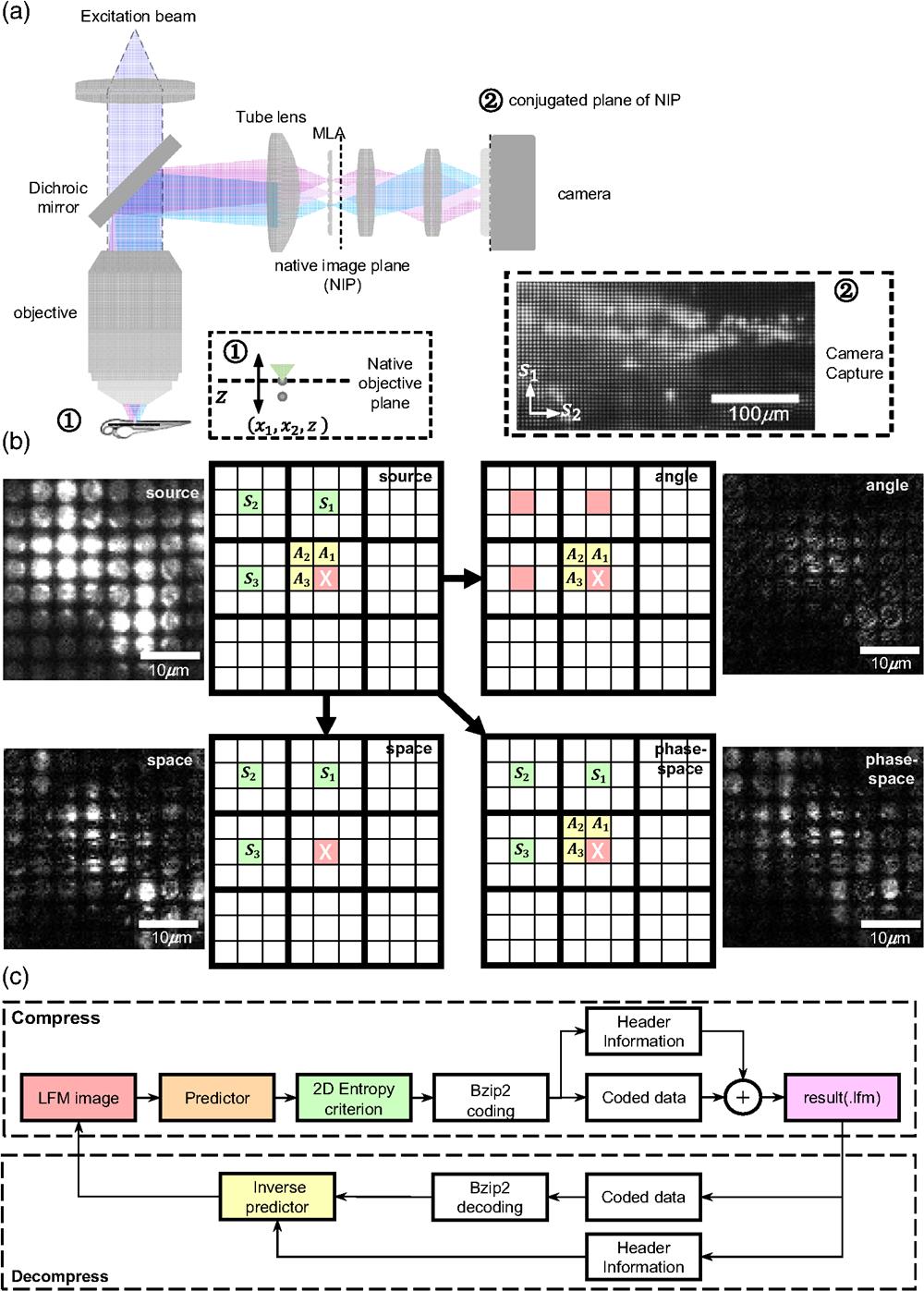
We built a light field fluorescence microscope based on a wide-field microscope by inserting a microlens array into the image plane of the tube lens [Fig. 1(a)]. In this way, the light field of the sample will be formed behind the microlens array, which then will be relayed to the image sensor for recording [Fig. 1(a)]. A sample zebrafish image captured by the light-field microscope shows the basic structure of the data. The LFM data has a 4D structure with not only spatial continuity but also angular continuity. Angular continuity characterizes the relationship between adjacent pixels in a microlens, while spatial continuity characterizes the relationship between adjacent microlens pixels at the same position. Traditional image compression algorithms mainly make predictions by using adjacent pixels. However, the predictors of a light field are no longer limited by this constraint.

In this case, the angular or spatial continuity can be applied alone for prediction. What is more, we can make full use of the continuity in both angular and spatial domains, which is named phase-space continuity, to make predictions for LFM data [Fig. 1(b)], thereby theoretically improving the compression ratio. Therefore, based on the phase-space continuity, we propose a PC-bzip2 compression framework for lossless LFM data compression [Fig. 1(c)]. The main idea of this framework is to add a prior knowledge-based predictor for the LFM data before the multicore CPU-accelerated bzip2 compression. In addition, we propose a two-dimensional (2D) image entropy criterion to determine which predictor is used to optimize the compression ratio. These two parts, as the preprocessing unit before bzip2 compression, can ensure that each compressed image has as little information redundancy as possible. Finally, the header information, including the selected predictor information and the coded data, can be packaged and stored in the file. In the decompression process, after multicore CPU-accelerated bzip2 decompression, we only need to select the corresponding inverse predictor according to the header information to restore the original LFM data (Fig. 1).

To sum up, the proposed PC-bzip2 lossless compression pipeline can be decomposed into four parts: prediction part, 2D image entropy criterion, multicore CPU accelerated bzip2 coding, and packing header information and coded data. We describe the details of each part in the following sections. The detailed schematic of the algorithm is shown in Fig. 1(c).

The prediction of pixel values leverages the interpixel continuity to reduce redundant information. Considering the 4D structure of light-field microscopy (LFM) data, characterized by 4D phase-space continuity, we separately predict the pixel value employing spatial continuity, angular continuity, and 4D phase-space continuity and compare their respective performances. When using spatial continuity exclusively, the pixel value is predicted by the neighboring pixels situated to the left, top, and top left. When employing angular continuity separately, the pixel value is predicted by the pixels in the same position from the neighboring microlenses located to the left, top, and top left. When incorporating 4D phase-space continuity, however, the predicted pixel value is not only related to neighboring pixels, but also influenced by those in adjacent microlenses. The schematic of these different predictors is shown in Fig. 1(b).

A 2D image entropy criterion is used to determine whether the prediction of pixel value will improve the compression ratio. As shown in Fig. 2, for the corresponding pixel, it not only has angle-adjacent pixels S1, S2, and S3, but also spatially adjacent pixels A1, A2, and A3. Therefore, the value of pixel S can be predicted by considering both these continuities. This process can be simply expressed as P(X)=Γi(S1,S2,S3,A1,A2,A3),(1)where P(X) is the predicted value, Γi represents the i’th predictor (predictor A corresponds to the first predictor, while predictor (A+B)/2 corresponds to the seventh predictor), as shown in Fig. 2(c). After applying the predictor to the input LFM image, the predicted image is obtained. Then we calculate the difference between the predicted image and the original image, yielding a 16-bit difference image, which can be formulated as I16−(u)=I16raw(u)−I16pre(u),(2)where I16raw(u) is the value of pixel u in the 16-bit original image I16raw), I16pre(u)=P(u) is the value of pixel u in the 16-bit predicted image I16pre, and I16−(u) is the value of pixel u in the 16-bit difference image. For further storage convenience, we map the value of I16−(u) to positive numbers Q16[I16−(u)], using odd numbers to represent positive values and even numbers to represent negative values. This can be mathematically described as Q16[I16−(u)]={2*|I16−(u)|−1,I16−(u)<02*|I16−(u)|,I16−(u)≥0.(3)

We further realign the 16-bit predicted image as an 8-bit data string and do a GPU-accelerated Burrows-Wheeler transform (BWT) on the 8-bit data string, which can be expressed as S8(m,n)=BWTAC{R8{Q16[I16−(u)]}},(4)where S8(m,n) is the characters at positions m and n in the 8-bit data string S8, R8 is the operator to realign 16-bit data to 8-bit, and BWTAC is the GPU-accelerated BWT. BWTAC is slightly different from the general BWT. From input to output, the general BWT includes three main steps: generating all rotations, sorting all rotations into lexical order, and taking the last column of all rotations. Different from the general BWT, when sorting all rotations, the GPU-accelerated BWT only considers the first character of each rotation. And if the first character of two rotations is the same, we keep the sorting order of these two rotations consistent with the generation. In this way, parallel acceleration can be achieved, and the time to determine whether the prediction is effective can be greatly reduced. After that, the 2D image entropy of the transformed data is calculated. Here, we suppose the transformed 8-bit data string as S8=[x1,x2,…,xn] (x1 is an 8-bit integer). In order to retain the sequential information of adjacent characters in the data, which is an essential part of move-to-front transform in the subsequent compression, we combine two adjacent 8-bit integers into a 16-bit integer, i.e., the data string is converted to a 16-bit data string S16=[x1x2,x2x3,…,xn−1xn] (xn−1xn is a 16-bit integer). Then, the 2D image entropy of the transformed 8-bit data string E(S8) could be calculated as E(S8)=∑65535t=0Ptn−1log(Ptn−1),(5)where t is the value of a 16-bit integer in S16, Pt represents the frequency of 16-bit integer value t, and n is the length of an 8-bit data string S8. A detailed schematic of the fast calculation of 2D image entropy is shown in Fig. 3. Subsequently, we evaluate the compression performance of each predictor’s output using 2D image entropy and identify the predictor with the lowest 2D image entropy as the final predictor. This operation can be expressed as i=F(min{Ei}),i∈{0,1,…,7},(6)where i corresponds to the index of the predictor with the best-estimated compression performance, Ei represents the value of 2D entropy when the predictor is the i’th (with the 0’th predictor indicating no predictor), and F(*) is used to locate the corresponding index for the value.

After validating the effectiveness of the prediction in enhancing compression ratio through 2D image entropy, the predicted image is then compressed utilizing the multicore CPU accelerated bzip2 algorithm. We reused the KLB code for our own purpose.7 KLB is currently one of the most advanced methods for bzip2 acceleration. The main idea of KLB is to split data into multiple blocks and then compress them in parallel, getting the utmost out of the multicore design of advanced computers. The KLB compression process consists of three steps. First, the data to be compressed is divided into some blocks. The block number corresponds to the number of threads supported by the computer processor, representing the maximum number of parallel operations. Second, multiple blocks are simultaneously compressed using the bzip2 algorithm, which is the main reason for the speed improvement of KLB compared to general bzip2. Finally, the compression results of each block in the previous step are written into the output file in turn, with the relevant information of the image and the block packed at the same time. Since we use different predictors for different images according to the 2D image entropy judgment result, we need to pack the predictor information into the final compressed file. Here, the predictor information is represented by an 8-bit unsigned integer in the header information of the final compressed file. The mapping table of predictors can be viewed in Fig. 2.

We investigated different predictors in the compression algorithm. The schematic of the LFM data is shown in Fig. 2(a). Among the seven types of predictors mainly applied in traditional compression methods (such as PNG and JPEG), four of them utilize more than one adjacent pixel for predictor calculation [Fig. 2(b)]. We then extend these predictors to the LFM data [Fig. 2(c)], including angle prediction, space prediction, and phase-space prediction.

To verify the performance of our PC-bzip2 compression experimentally, we imaged the fluorescent beads and MCF-10A cells separately with the LFM under the different exposure times [Fig. 4(a)], where the image of the fluorescent beads represents typical LFM data without continuous structural information, while the image of the MCF-10A cells represents a typical LFM data with better structural information. Different exposure times will cause images to have different SNRs. Then we tested the performance of all the phase-space predictors [Figs. 2(b) and 2(c)] on these two types of LFM images with different SNRs. We find that as the image SNR increases (i.e., more information is detected within the image), the compression ratio gradually increases, which means the increase in the number of bits required for each dimension for all the predictors [Figs. 4(b) and 4(c)]. For the images of the fluorescent beads without continuous structural information, the prediction step did not improve the final compression ratio [Fig. 4(c)]. But for the MCF-10A cells images with better continuous structure information, the prediction step can significantly increase the final compression rate [Fig. 4(b)] and the maximum improvement can reach 0.77 bits/dim.

In the compression tests of both fluorescent bead images and MCF-10A cell images, the 2D entropy criterion can accurately predict the optimal predictors with the optimal compression ratios [Fig. 4(b) and 4(c)]. In addition, we further tested the predictor (B+(A−C)/2) using angle prediction, space prediction, and phase-space prediction separately [Fig. 4(d)], and the phase-space predictor showed the highest compression ratio. In addition, to further demonstrate the enhancement of the compression ratio in our PC-bzip2, we compared our PC-bzip2 with KLB on the images of MCF-10A in terms of time consumption (including compression and decompression) and compression rate. With almost no additional time consumption, the compression ratio can be increased by 10% [Fig. 4(e)]. This tiny time gap can be further reduced with the upgrade of the GPU.

Since the recording of biological dynamic processes such as neuron activity by LFM usually lasts for a long time with a high frame rate, massive quantities of time series data will consequently be generated. Therefore, we have extended our method to the time dimension to further improve its practicality (Fig. S2 in the Supplementary Material). When performing lossless compression on time series LFM data, we consider introducing the temporal continuity into the basis of original 4D phase-space continuity. First, in order to find the best predictor for a single frame, the first frame is processed according to the compression method of PC-bzip2 [Fig. 1(c)], where the result of the 2D entropy criterion will be used as the main predictor in the subsequent frames. For the subsequent frames, we introduce the interframe predictor combined with the single-image predictor to further reduce redundant information in time series data (Fig. S3 in the Supplementary Material). Once the predictor for a single image is determined by the first frame, all subsequent frames will be predicted by introducing temporal continuity on the basis of this predictor. After all the time series data are predicted and symbolized, the result will be divided into several blocks (equal to the maximum number of threads supported by the computer), and then compressed by bzip2 in parallel. The compression result and header information are written to the file.

To verify the advantage of the extension method, we imaged the live larval zebrafish by recording 20 frames of the heartbeat of the zebrafish under different exposure times [Fig. 5(a)], which will be later compressed in the separate use of spatial continuity, angular continuity, phase-space continuity, and their respective expansions in the time dimension. Introducing the time continuity into the predictor is beneficial for the improvement of compression ratios [Fig. 5(b)]. Without time continuity, the compression ratio using the spatial predictor is better than that using the angular predictor. On the contrary, the method of angular predictor combined with time continuity is better, which means that the angular continuity is higher than the spatial continuity in the time dimension. Compared with only keeping the phase-space continuity, our method could realize higher compression ratios by combining with the time continuity [Fig. 5(c)]. We also compared our methods with the state-of-the-art lossless compression method KLB. Whether or not in combination with temporal continuity, our methods could be significantly better than KLB in the compression ratio [Fig. 5(c)]. Comparing the compression results under different SNRs, it can be seen that the final compression ratios mainly depend on the amount of information contained in the video. To demonstrate the truly lossless compression of our method on time series, we perform local statistics on the images randomly selected from the decompressed time series under different SNRs [Figs. 6(c) and 6(d)], showing that our method achieves the really lossless compression and decompression processes whether in the intuitive vision of the image or its specific distribution.

In order to visually demonstrate the performance of our PC-bzip2 method in generalizing to different data formats, including image data and time series (video) data, we show multiple sets of comparison of the images and their gray-scale performance before and after PC-bzip2 compression in Fig. 6. We first compared the decompressed larval zebrafish image compressed by B3D and PC-bzip2, indicating that our method can realize truly lossless compression [Fig. 6(a)] Then we compared the decompressed image of MCF-10A image data [Fig. 6(b)] compressed by our PC-bzip2 with its original images. Similarly, we also compared the images from the time series zebrafish data of different excitation powers [Figs. 6(c) and 6(d)]. The results demonstrated the ability of our PC-bzip2 to achieve efficient lossless compression and decompression performance for both image data and time series image data.

We have developed a 4D phase-space continuity-enhanced bzip2 lossless compression method to realize high-speed and efficient LFM data compression. By adding a suitable predictor determined by the 2D image entropy criterion before bzip2 or KLB compression, we achieved almost 10% improvement in compression ratio with a little increase in time. We demonstrated the performance of the PC-bzip2 algorithm on fluorescence beads data and cells data with different SNRs. Since the recording of multicellular organisms by LFM usually generates huge time series data, we further extended our method to the time dimension to improve its practicality. We validate the temporal extension of PC-bzip2 on time series recording of zebrafish blood vessels. Compared to the predictor in the traditional compression method, we fully exploited the structure of LFM image or video to achieve high compression performance. We provided a fast MATLAB interface, and an ImageJ plug-in was provided for ease of use. The PC-bzip2 can become a promising and lightweight tool for any light-field microscope.

Since the improvement of compression ratio in PC-bzip2 is mainly determined by the redundancy of LFM data, the PC-bzip2 algorithm will not show significant improvement on all samples. Therefore, in our method, we use the 2D image entropy criterion to choose a suitable predictor or directly apply the bzip2 compression algorithm without a predictor for the adaption to different samples. Further improvement may include extending the algorithm to the spectral dimension and optimizing the time consumption of the 2D image entropy criterion. We believe such improvements in compression performance will bring advanced data storage capacity with a lightweight tool to the broad microscopic community, facilitating mass data storage and processing in various biomedical applications like multicellular organism observation.

Bo Xiong is a postdoc at Peking University. He received his BS and PhD degrees in control science and engineering from Tsinghua University in 2015 and 2022, respectively. He is the author of more than 10 journal papers. His current research interests include computational imaging & microscopy, and neuromorphic vision. He is a member of OPTICA and IEEE.

Biographies of the other authors are not available.

References

[10] Y. Bai et al. Deep lossy plus residual coding for lossless and near-lossless image compression. IEEE Trans. Pattern. Anal. Mach. Intell., 1-18(2024).
[11] K. K. Shukla, M. Prasad. Lossy Image Compression: Domain Decomposition-Based Algorithms(2011).
[12] M. Rabbani, P. W. Jones. Digital Image Compression Techniques(1991).
[15] M. Lu et al. Transformer-based image compression, 469-469(2022).
[16] Y. Qian et al. Entroformer: a transformer-based entropy model for learned image compression(2021).
[17] D. W. Cromey. Digital images are data: and should be treated as such. Cell Imaging Technol. Methods. Protoc., 931, 1-27(2013).
[21] S. Radhakrishnan, L. M. Matos, A. J. Neves, A. J. Pinho. Lossy-to-lossless compression of biomedical images based on image decomposition. Applications of Digital Signal Processing through Practical Approach(2015).
[24] B. Balázs et al. A real-time compression library for microscopy images(2017).
[26] J. Townsend, T. Bird, D. Barber. Practical lossless compression with latent variables using bits back coding, 7(2020).
[27] J. Townsend et al. Hilloc: lossless image compression with hierarchical latent variable models, 7(2019).
[29] F. Kingma, P. Abbeel, J. Ho. Bit-swap: recursive bits-back coding for lossless compression with hierarchical latent variables, 3408-3417(2019).
[30] J. Ho, E. Lohn, P. Abbeel. Compression with flows via local bits-back coding(2019).
[31] I. Goodfellow et al. Generative adversarial nets(2014).
[32] F. Mentzer et al. High-fidelity generative image compression, 11913-11924(2020).
[33] L. Wu, K. Huang, H. Shen. A GAN-based tunable image compression system, 2334-2342(2020).
[35] E. Hoogeboom et al. Integer discrete flows and lossless compression(2019).
[41] R. van den Berg et al. IDF++: analyzing and improving integer discrete flows for lossless compression(2020).
[43] S. Zhang et al. iFlow: numerically invertible flows for efficient lossless compression via a uniform coder, 5822-5833(2021).
Set citation alerts for the article
Please enter your email address
© Copyright 2018-2021 | Chinese Laser Press. All Rights Reserved 沪ICP备15018463号-20